


注意
跳到文末可下载完整示例源码。
与其他图形软件包一样,Matplotlib建立在变换框架之上,可以方便地在用户数据坐标、Axes坐标、Figure坐标和显示坐标之间转换。在95%的绘图任务中,这些操作在底层自动完成,无需专门考虑;但当你深入定制图形时,理解这些对象会帮助你复用Matplotlib提供的变换,或者创建自己的变换,参见matplotlib.transforms。下表概括了常用坐标系、含义及其转换到显示坐标的变换对象。“变换对象”一列中,ax是Axes实例,fig是Figure实例,subfigure是SubFigure实例。
|
坐标系 |
说明 |
从该坐标系到显示坐标的变换对象 |
|---|---|---|
|
data(数据坐标) |
Axes内数据使用的坐标系。 |
|
|
axes(Axes坐标) |
Axes的坐标系: |
|
|
subfigure(子图形坐标) |
SubFigure的坐标系: |
|
|
figure(图形坐标) |
Figure的坐标系: |
|
|
figure-inches(图形英寸坐标) |
Figure的英寸坐标系: |
|
|
xaxis、yaxis |
混合坐标系:一个方向使用数据坐标,另一个方向使用Axes坐标。 |
|
|
display(显示坐标) |
输出的原生坐标系: 显示单位取决于后端:例如Agg使用像素,SVG和PDF使用点。 |
Transform对象本身并不知道输入与输出属于哪种坐标系,不过上表中的对象都被构造为接受相应坐标系中的输入,并转换为显示坐标。因此显示坐标这一行的“变换对象”为None:它已经处于显示坐标中。这些命名与目标坐标约定有助于理解已有的标准坐标系与变换。
变换还能通过Transform.inverted生成逆变换,将输出坐标转换回输入坐标。例如,ax.transData把数据坐标转换为显示坐标,而ax.transData.inverted()是从显示坐标转换回数据坐标的matplotlib.transforms.Transform。这对于处理用户界面事件尤其有用:事件通常发生在显示空间,而你希望知道鼠标点击或按键在数据坐标系中的位置。
如果用显示坐标指定Artist的位置,图形的DPI或尺寸变化可能改变它们的相对位置。这会在打印或更改屏幕分辨率时造成困惑,因为对象的位置与大小都可能变化。因此,在Axes或Figure中放置Artist时,通常会将变换设为IdentityTransform()之外的对象。使用add_artist将Artist加入Axes时,默认变换是ax.transData,这样可以用数据坐标思考和操作,由Matplotlib负责转换到显示坐标。
数据坐标
先从最常用的数据坐标系开始。每当向Axes添加数据时,Matplotlib都会更新数据范围,常见方式是调用set_xlim()和set_ylim()。下图的x轴范围为0到10,y轴范围为−1到1。
import matplotlib.pyplot as plt
import numpy as np

import matplotlib.patches as mpatches

x = np.arange(0, 10, 0.005)
y = np.exp(-x/2.) * np.sin(2*np.pi*x)

fig, ax = plt.subplots()
ax.plot(x, y)
ax.set_xlim(0, 10)
ax.set_ylim(-1, 1)

plt.show()
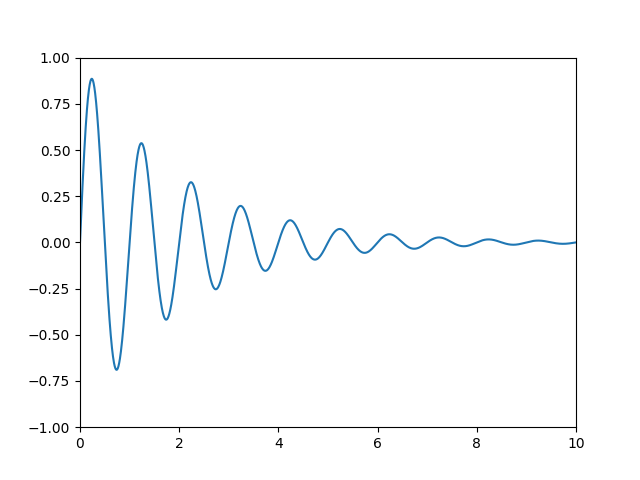
可以用ax.transData把数据坐标转换为显示坐标,输入既可以是单个点,也可以是点序列:
In [14]: type(ax.transData)
Out[14]: <class 'matplotlib.transforms.CompositeGenericTransform'>

In [15]: ax.transData.transform((5, 0))
Out[15]: array([ 335.175,  247.   ])

In [16]: ax.transData.transform([(5, 0), (1, 2)])
Out[16]:
array([[ 335.175,  247.   ],
       [ 132.435,  642.2  ]])
可以使用inverted()创建从显示坐标转换回数据坐标的变换:
In [41]: inv = ax.transData.inverted()

In [42]: type(inv)
Out[42]: <class 'matplotlib.transforms.CompositeGenericTransform'>

In [43]: inv.transform((335.175,  247.))
Out[43]: array([ 5.,  0.])
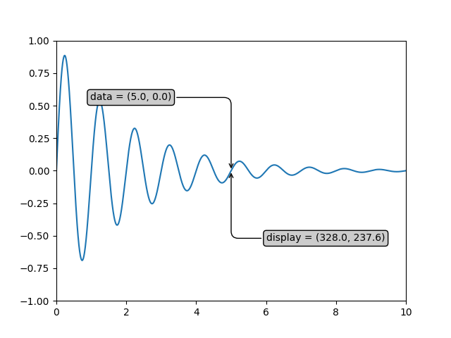
如果跟着本教程输入代码,不同的窗口尺寸或DPI设置可能使显示坐标值不同。下图标注的显示坐标也可能与IPython会话不同,因为文档图形使用不同的默认尺寸。
x = np.arange(0, 10, 0.005)
y = np.exp(-x/2.) * np.sin(2*np.pi*x)

fig, ax = plt.subplots()
ax.plot(x, y)
ax.set_xlim(0, 10)
ax.set_ylim(-1, 1)

xdata, ydata = 5, 0
# This computing the transform now, if anything
# (figure size, dpi, axes placement, data limits, scales..)
# changes re-calling transform will get a different value.
xdisplay, ydisplay = ax.transData.transform((xdata, ydata))

bbox = dict(boxstyle="round", fc="0.8")
arrowprops = dict(
    arrowstyle="->",
    connectionstyle="angle,angleA=0,angleB=90,rad=10")

offset = 72
ax.annotate(f'data = ({xdata:.1f}, {ydata:.1f})',
            (xdata, ydata), xytext=(-2*offset, offset), textcoords='offset points',
            bbox=bbox, arrowprops=arrowprops)

disp = ax.annotate(f'display = ({xdisplay:.1f}, {ydisplay:.1f})',
                   (xdisplay, ydisplay), xytext=(0.5*offset, -offset),
                   xycoords='figure pixels',
                   textcoords='offset points',
                   bbox=bbox, arrowprops=arrowprops)

plt.show()
警告
在GUI后端运行上述源码时,可能发现数据标注与显示标注的箭头没有指向完全相同的位置。原因是显示坐标在图形实际展示前计算,而GUI后端可能在创建窗口时稍微调整图形尺寸;手动调整窗口大小后,差异会更明显。这也是很少直接使用显示空间的原因之一。不过,可以连接on_draw事件,在绘制时更新图形坐标,详见事件处理与拾取。
改变坐标轴的x或y范围后,数据范围更新,变换也就产生新的显示坐标。仅修改ylim时,只有显示坐标的y分量改变;再修改xlim时,两个分量都改变。后面介绍Bbox时还会进一步讨论。
In [54]: ax.transData.transform((5, 0))
Out[54]: array([ 335.175,  247.   ])

In [55]: ax.set_ylim(-1, 2)
Out[55]: (-1, 2)

In [56]: ax.transData.transform((5, 0))
Out[56]: array([ 335.175     ,  181.13333333])

In [57]: ax.set_xlim(10, 20)
Out[57]: (10, 20)

In [58]: ax.transData.transform((5, 0))
Out[58]: array([-171.675     ,  181.13333333])
Axes坐标
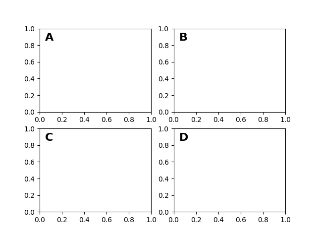
除数据坐标外,Axes坐标可能是第二常用的坐标系。在其中,(0, 0)是Axes或子图左下角,(0.5, 0.5)是中心,(1.0, 1.0)是右上角。也可引用范围外的点,例如(−0.1, 1.1)位于Axes的左上方。这在放置文字时特别有用:你可能希望文字框固定在Axes面板左上角,并在平移或缩放后仍保持该位置。下面的简单示例创建四个面板,并按期刊常见方式标记为A、B、C、D。更完善的方法见为子图添加标签。
fig = plt.figure()
for i, label in enumerate(('A', 'B', 'C', 'D')):
    ax = fig.add_subplot(2, 2, i+1)
    ax.text(0.05, 0.95, label, transform=ax.transAxes,
            fontsize=16, fontweight='bold', va='top')

plt.show()
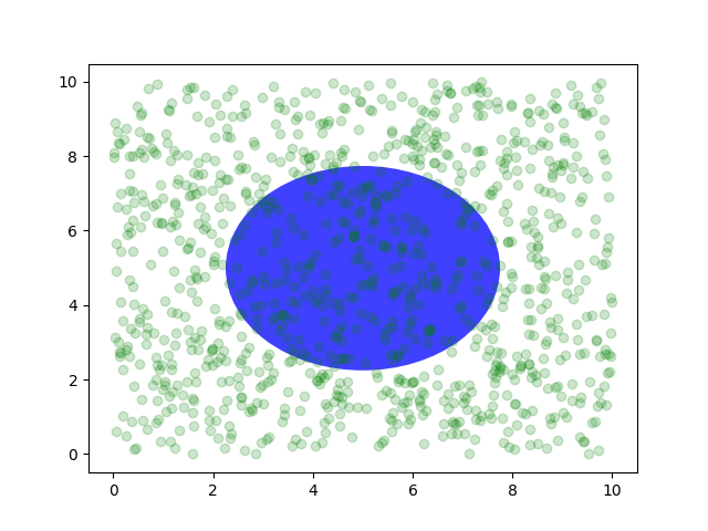
也可以在Axes坐标中绘制线条或patch,但原作者认为,这通常不如用ax.transAxes放置文字有用。下面是一个简单示例:在数据空间中绘制随机点,再叠加一个以Axes中心为圆心、半径为Axes四分之一的半透明Circle。若Axes没有保持纵横比,参见set_aspect(),它看起来会像椭圆。使用平移、缩放工具或手动改变xlim与ylim后,数据会移动,但圆仍固定在Axes中心,因为它并不使用数据坐标。
fig, ax = plt.subplots()
x, y = 10*np.random.rand(2, 1000)
ax.plot(x, y, 'go', alpha=0.2)  # plot some data in data coordinates

circ = mpatches.Circle((0.5, 0.5), 0.25, transform=ax.transAxes,
                       facecolor='blue', alpha=0.75)
ax.add_patch(circ)
plt.show()
混合变换
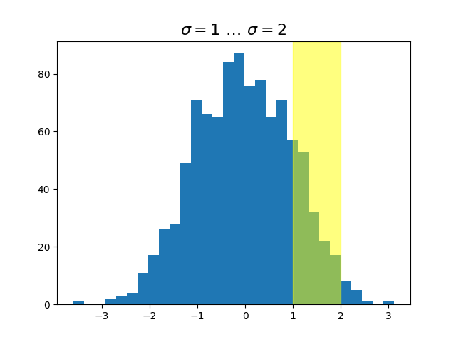
混合Axes坐标和数据坐标非常有用,例如突出某个y数据区间的水平带:无论数据范围、平移或缩放如何变化,它始终覆盖整个x轴。此类线条与区域非常常用,因此Matplotlib提供了axhline()、axvline()、axhspan()和axvspan()。为说明原理,这里用混合变换自行实现水平区域。此技巧只适用于普通笛卡尔坐标系那样的可分离变换,不适用于PolarTransform等不可分离变换。
import matplotlib.transforms as transforms

fig, ax = plt.subplots()
x = np.random.randn(1000)

ax.hist(x, 30)
ax.set_title(r'$\sigma=1 \/ \dots \/ \sigma=2$', fontsize=16)

# the x coords of this transformation are data, and the y coord are axes
trans = transforms.blended_transform_factory(
    ax.transData, ax.transAxes)
# highlight the 1..2 stddev region with a span.
# We want x to be in data coordinates and y to span from 0..1 in axes coords.
rect = mpatches.Rectangle((1, 0), width=1, height=1, transform=trans,
                          color='yellow', alpha=0.5)
ax.add_patch(rect)

plt.show()
注意
x方向用数据坐标、y方向用Axes坐标的混合变换非常常用,因此Matplotlib提供辅助方法,返回内部绘制刻度和刻度标签时所用的变换:matplotlib.axes.Axes.get_xaxis_transform()与matplotlib.axes.Axes.get_yaxis_transform()。因此,上例中blended_transform_factory()的调用可以替换为get_xaxis_transform:
trans = ax.get_xaxis_transform()
使用物理坐标绘图
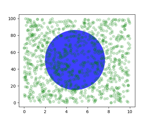
有时希望图中对象具有确定的物理尺寸。下面绘制与前面相同的圆,但使用物理坐标。交互操作时可以看到:改变图形尺寸并不会改变圆到左下角的偏移,也不会改变圆的大小;无论Axes纵横比如何,它都保持为圆。
fig, ax = plt.subplots(figsize=(5, 4))
x, y = 10*np.random.rand(2, 1000)
ax.plot(x, y*10., 'go', alpha=0.2)  # plot some data in data coordinates
# add a circle in fixed-coordinates
circ = mpatches.Circle((2.5, 2), 1.0, transform=fig.dpi_scale_trans,
                       facecolor='blue', alpha=0.75)
ax.add_patch(circ)
plt.show()
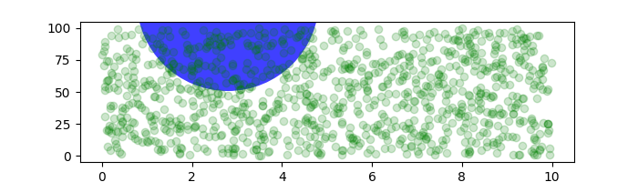
改变图形尺寸后,圆的绝对位置不变,并会被裁剪。
fig, ax = plt.subplots(figsize=(7, 2))
x, y = 10*np.random.rand(2, 1000)
ax.plot(x, y*10., 'go', alpha=0.2)  # plot some data in data coordinates
# add a circle in fixed-coordinates
circ = mpatches.Circle((2.5, 2), 1.0, transform=fig.dpi_scale_trans,
                       facecolor='blue', alpha=0.75)
ax.add_patch(circ)
plt.show()
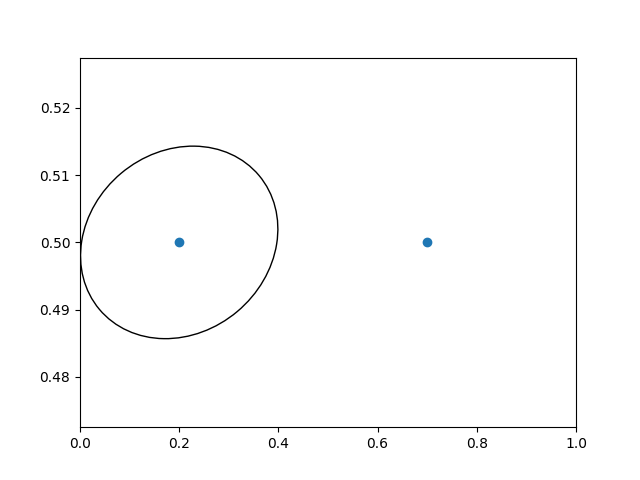
另一种用途是在Axes中的某个数据点周围放置具有固定物理尺寸的patch。这里组合两个变换:第一个决定椭圆大小,第二个决定位置。先将椭圆放在原点,再通过辅助变换ScaledTranslation,将它移动到ax.transData坐标系中的正确位置。该辅助对象的实例化形式为:
trans = ScaledTranslation(xt, yt, scale_trans)
其中xt与yt是平移偏移量,scale_trans是在应用偏移之前、于变换时缩放这两个偏移量的变换。
请注意下面变换对象之间的加号。它表示先应用fig.dpi_scale_trans缩放,使椭圆获得正确尺寸,但仍以(0, 0)为中心;然后在数据空间中平移到xdata[0]和ydata[0]。
交互使用时,即使通过缩放改变坐标轴范围,椭圆仍保持相同尺寸。
fig, ax = plt.subplots()
xdata, ydata = (0.2, 0.7), (0.5, 0.5)
ax.plot(xdata, ydata, "o")
ax.set_xlim(0, 1)

trans = (fig.dpi_scale_trans +
         transforms.ScaledTranslation(xdata[0], ydata[0], ax.transData))

# plot an ellipse around the point that is 150 x 130 points in diameter...
circle = mpatches.Ellipse((0, 0), 150/72, 130/72, angle=40,
                          fill=None, transform=trans)
ax.add_patch(circle)
plt.show()
注意
变换顺序很重要。这里先在显示空间赋予椭圆正确尺寸,再在数据空间移动到正确位置。如果先执行ScaledTranslation,xdata[0]与ydata[0]会先转换为显示坐标,例如200 DPI显示器上的[358.4 475.2];随后再被fig.dpi_scale_trans缩放,椭圆中心就会远离屏幕,变成[71680. 95040.]。
使用偏移变换创建阴影
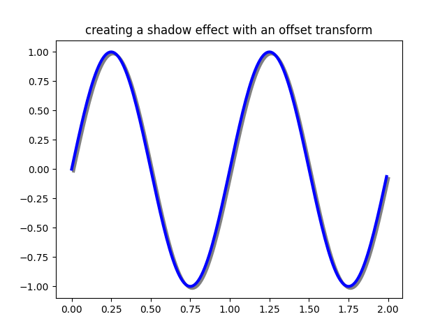
ScaledTranslation还可以创建相对于已有变换具有偏移的新变换,例如让一个对象相对另一个对象稍微移动。通常希望这种偏移以点或英寸等物理单位表达,而非数据坐标,使其在不同缩放级别和DPI下保持一致。
偏移的一种用途是阴影:绘制一个与原对象相同、稍向右下方移动的对象,并调整zorder,确保先绘制阴影,再在其上绘制原对象。
这里应用变换的顺序与前面ScaledTranslation示例相反:先使用ax.transData在数据坐标中绘图,再通过fig.dpi_scale_trans以dx、dy点为单位偏移。排版中的一个点为1/72英寸。以点指定偏移,就能在保存图形时保持相同外观,不受DPI分辨率影响。
fig, ax = plt.subplots()

# make a simple sine wave
x = np.arange(0., 2., 0.01)
y = np.sin(2*np.pi*x)
line, = ax.plot(x, y, lw=3, color='blue')

# shift the object over 2 points, and down 2 points
dx, dy = 2/72., -2/72.
offset = transforms.ScaledTranslation(dx, dy, fig.dpi_scale_trans)
shadow_transform = ax.transData + offset

# now plot the same data with our offset transform;
# use the zorder to make sure we are below the line
ax.plot(x, y, lw=3, color='gray',
        transform=shadow_transform,
        zorder=0.5*line.get_zorder())

ax.set_title('creating a shadow effect with an offset transform')
plt.show()
注意
DPI和英寸偏移很常见,因此有专门的辅助函数matplotlib.transforms.offset_copy(),返回附加了偏移的新变换。上例也可以写为:
shadow_transform = transforms.offset_copy(ax.transData,
         fig, dx, dy, units='inches')
变换流水线
本教程使用的ax.transData由三个变换组成,共同构成从数据坐标到显示坐标的流水线。Michael Droettboom实现了这套框架,提供清晰API,将极坐标图和对数图中的非线性投影及缩放,与平移、缩放时的线性仿射变换分离。这提高了效率:平移和缩放Axes只影响仿射变换,不一定需要在简单导航事件中重新计算较昂贵的非线性缩放或投影。仿射变换矩阵还可以先相乘,再一次性应用于坐标;并非所有变换都具有这种性质。
基础的可分离坐标轴Axes类中,ax.transData实例定义如下:
self.transData = self.transScale + (self.transLimits + self.transAxes)
在前面的Axes坐标一节已介绍transAxes:它把Axes或子图边界框的(0, 0)与(1, 1)角点映射到显示空间。下面来看另外两部分。
self.transLimits把数据坐标变为Axes坐标,也就是将视图的xlim和ylim映射到Axes的单位空间,再由transAxes映射到显示空间。下面可以看到这一过程:
In [80]: ax = plt.subplot()

In [81]: ax.set_xlim(0, 10)
Out[81]: (0, 10)

In [82]: ax.set_ylim(-1, 1)
Out[82]: (-1, 1)

In [84]: ax.transLimits.transform((0, -1))
Out[84]: array([ 0.,  0.])

In [85]: ax.transLimits.transform((10, -1))
Out[85]: array([ 1.,  0.])

In [86]: ax.transLimits.transform((10, 1))
Out[86]: array([ 1.,  1.])

In [87]: ax.transLimits.transform((5, 0))
Out[87]: array([ 0.5,  0.5])
也可以使用同一个逆变换,从单位Axes坐标回到数据坐标。
In [90]: inv.transform((0.25, 0.25))
Out[90]: array([ 2.5, -0.5])
最后是self.transScale,负责可选的数据非线性缩放,例如对数坐标轴。Axes刚建立时,默认使用线性刻度,因此它是恒等变换。当调用semilogx()等对数缩放函数,或通过set_xscale()显式设置对数刻度后,ax.transScale会负责非线性映射。刻度变换分别属于xaxis和yaxis的Axis实例。例如,调用ax.set_xscale('log')时,xaxis会将自己的刻度更新为matplotlib.scale.LogScale实例。
不可分离坐标轴还有其他部分需要考虑,尤其是投影变换。例如,matplotlib.projections.polar.PolarAxes的transData比普通可分离Axes复杂:
self.transData = (
    self.transScale + self.transShift + self.transProjection +
    (self.transProjectionAffine + self.transWedge + self.transAxes))
transProjection负责将数据坐标,例如地图中的经纬度、极坐标中的半径和角度,投影到可分离的笛卡尔坐标系。matplotlib.projections包含一些投影示例。由于Matplotlib支持扩展坐标轴和投影,进一步学习的好方法是查看这些包的源码,了解如何构造自己的投影。Michael Droettboom提供了创建Hammer投影坐标轴的教程示例,见自定义投影。
原文示例脚本总运行时间:0分3.825秒。
原文:变换教程;作者:Matplotlib开发团队与文档贡献者。版本或日期:Matplotlib3.11.2文档。原文及源码权利归相应权利人所有。
本文示例运行时间与图示均来自原文,不代表本文编者运行所得。











暂无评论内容