


这里所说的“分组”(group by),是指包含以下一个或多个步骤的处理过程:
- 拆分:根据某种规则将数据分成若干组。
- 应用:独立地对每一组应用函数。
- 合并:将结果组合成一种数据结构。
其中,拆分最为直接。在应用步骤中,我们可能需要执行以下操作:
- 聚合:为每组计算一个或多个汇总统计量。例如:
- 变换:执行组内计算,返回与原数据索引相同的对象。例如:
- 筛选:根据每组计算得到的 True 或 False 结果,丢弃部分组。例如:
GroupBy 对象定义了许多此类操作。它们与 聚合 API、窗口 API 和 重采样 API 的操作相似。
有些操作可能不属于这些类别,或者是几类操作的组合。这时可以考虑 GroupBy 的 apply 方法。它会检查应用步骤的结果;如果结果不属于上述三类,就尝试以合理方式合并为一个结果。
使用过 SQL 工具或 itertools 的读者,应该对 GroupBy 这个名称很熟悉。例如,SQL 可以这样写:
SELECT Column1, Column2, mean(Column3), sum(Column4)
FROM SomeTable
GROUP BY Column1, Column2
pandas 希望让这类操作的表达自然、简洁。下文会逐项介绍 GroupBy 的功能,再给出一些更复杂的示例与使用场景。
更多进阶策略见 实用配方。
将对象拆分为组
从抽象角度看,分组就是提供一个从标签到组名的映射。可以按以下方式创建 GroupBy 对象,稍后会进一步说明这种对象:
In [1]: speeds = pd.DataFrame(
   ...:     [
   ...:         ("bird", "Falconiformes", 389.0),
   ...:         ("bird", "Psittaciformes", 24.0),
   ...:         ("mammal", "Carnivora", 80.2),
   ...:         ("mammal", "Primates", np.nan),
   ...:         ("mammal", "Carnivora", 58),
   ...:     ],
   ...:     index=["falcon", "parrot", "lion", "monkey", "leopard"],
   ...:     columns=("class", "order", "max_speed"),
   ...: )
   ...:

In [2]: speeds
Out[2]:
          class           order  max_speed
falcon     bird   Falconiformes      389.0
parrot     bird  Psittaciformes       24.0
lion     mammal       Carnivora       80.2
monkey   mammal        Primates        NaN
leopard  mammal       Carnivora       58.0
In [3]: grouped = speeds.groupby("class")

In [4]: grouped = speeds.groupby(["class", "order"])
映射可以通过多种方式指定:
- Python 函数:对每个索引标签调用该函数。
- 与索引长度相同的列表或 NumPy 数组。
- 字典或
Series:提供标签 -> 组名的映射。
- 对于
DataFrame,可使用字符串指定用于分组的列名或索引层级名。
- 由上述任意对象组成的列表。
这些分组对象统称为键。例如,考虑下面的 DataFrame:
In [5]: df = pd.DataFrame(
   ...:     {
   ...:         "A": ["foo", "bar", "foo", "bar", "foo", "bar", "foo", "foo"],
   ...:         "B": ["one", "one", "two", "three", "two", "two", "one", "three"],
   ...:         "C": np.random.randn(8),
   ...:         "D": np.random.randn(8),
   ...:     }
   ...: )
   ...:

In [6]: df
Out[6]:
     A      B         C         D
0  foo    one  0.469112 -0.861849
1  bar    one -0.282863 -2.104569
2  foo    two -1.509059 -0.494929
3  bar  three -1.135632  1.071804
4  foo    two  1.212112  0.721555
5  bar    two -0.173215 -0.706771
6  foo    one  0.119209 -1.039575
7  foo  three -1.044236  0.271860
在 DataFrame 上调用 groupby() 可获得 GroupBy 对象,返回类型为 pandas.api.typing.DataFrameGroupBy。可以按 A 列、B 列或同时按这两列分组:
In [7]: grouped = df.groupby("A")

In [8]: grouped = df.groupby("B")

In [9]: grouped = df.groupby(["A", "B"])DataFrame 的 groupby 始终沿轴 0(行)操作。若希望按列拆分,应先转置:
In [10]: def get_letter_type(letter):
   ....:     if letter.lower() in 'aeiou':
   ....:         return 'vowel'
   ....:     else:
   ....:         return 'consonant'
   ....:

In [11]: grouped = df.T.groupby(get_letter_type)
pandas 的 Index 允许重复值。如果把非唯一索引用作分组键,相同索引值对应的所有记录都属于同一组,因此聚合结果只包含唯一的索引值:
In [12]: index = [1, 2, 3, 1, 2, 3]

In [13]: s = pd.Series([1, 2, 3, 10, 20, 30], index=index)

In [14]: s
Out[14]:
1     1
2     2
3     3
1    10
2    20
3    30
dtype: int64

In [15]: grouped = s.groupby(level=0)

In [16]: grouped.first()
Out[16]:
1    1
2    2
3    3
dtype: int64

In [17]: grouped.last()
Out[17]:
1    10
2    20
3    30
dtype: int64

In [18]: grouped.sum()
Out[18]:
1    11
2    22
3    33
dtype: int64
真正需要时才会发生拆分。创建 GroupBy 对象只会验证传入的映射是否有效。
GroupBy 的排序
默认情况下,groupby 会对分组键排序。传入 sort=False 可能提高速度;这时组键的顺序遵循它们在原 DataFrame 中首次出现的顺序:
In [19]: df2 = pd.DataFrame({"X": ["B", "B", "A", "A"], "Y": [1, 2, 3, 4]})

In [20]: df2.groupby(["X"]).sum()
Out[20]:
   Y
X
A  7
B  3

In [21]: df2.groupby(["X"], sort=False).sum()
Out[21]:
   Y
X
B  3
A  7
groupby 会保留每组内部记录的原有顺序。例如,下例各组中的记录顺序与它们在原 DataFrame 中出现的顺序一致:
In [22]: df3 = pd.DataFrame({"X": ["A", "B", "A", "B"], "Y": [1, 4, 3, 2]})

In [23]: df3.groupby("X").get_group("A")
Out[23]:
   X  Y
0  A  1
2  A  3

In [24]: df3.groupby(["X"]).get_group(("B",))
Out[24]:
   X  Y
1  B  4
3  B  2
GroupBy 的 dropna
默认情况下,分组键中的 NA 值会被排除。若希望把 NA 也纳入分组键,可传入 dropna=False。
In [25]: df_list = [[1, 2, 3], [1, None, 4], [2, 1, 3], [1, 2, 2]]

In [26]: df_dropna = pd.DataFrame(df_list, columns=["a", "b", "c"])

In [27]: df_dropna
Out[27]:
   a    b  c
0  1  2.0  3
1  1  NaN  4
2  2  1.0  3
3  1  2.0  2
# Default ``dropna`` is set to True, which will exclude NaNs in keys
In [28]: df_dropna.groupby(by=["b"], dropna=True).sum()
Out[28]:
     a  c
b
1.0  2  3
2.0  2  5

# In order to allow NaN in keys, set ``dropna`` to False
In [29]: df_dropna.groupby(by=["b"], dropna=False).sum()
Out[29]:
     a  c
b
1.0  2  3
2.0  2  5
NaN  1  4
dropna 参数的默认值是 True,表示分组键不包含 NA。
GroupBy 对象的属性
GroupBy 对象的 groups 属性是一个字典,将每个唯一分组键映射到该组包含的索引标签。以上例来说:
In [30]: df.groupby("A").groups
Out[30]: {'bar': [1, 3, 5], 'foo': [0, 2, 4, 6, 7]}

In [31]: df.T.groupby(get_letter_type).groups
Out[31]: {'consonant': ['B', 'C', 'D'], 'vowel': ['A']}
对 GroupBy 对象调用 Python 标准函数 len,会返回组的数量,与 groups 字典的长度相同:
In [32]: grouped = df.groupby(["A", "B"])

In [33]: grouped.groups
Out[33]:
{('bar', 'one'): RangeIndex(start=1, stop=2, step=1),
 ('bar', 'three'): RangeIndex(start=3, stop=4, step=1),
 ('bar', 'two'): RangeIndex(start=5, stop=6, step=1),
 ('foo', 'one'): RangeIndex(start=0, stop=12, step=6),
 ('foo', 'three'): RangeIndex(start=7, stop=8, step=1),
 ('foo', 'two'): RangeIndex(start=2, stop=6, step=2)}

In [34]: len(grouped)
Out[34]: 6
GroupBy 支持对列名、GroupBy 操作及其他属性进行 Tab 补全:
In [35]: n = 10

In [36]: weight = np.random.normal(166, 20, size=n)

In [37]: height = np.random.normal(60, 10, size=n)

In [38]: time = pd.date_range("1/1/2000", periods=n)

In [39]: gender = np.random.choice(["male", "female"], size=n)

In [40]: df = pd.DataFrame(
   ....:     {"height": height, "weight": weight, "gender": gender}, index=time
   ....: )
   ....:

In [41]: df
Out[41]:
               height      weight  gender
2000-01-01  42.849980  157.500553    male
2000-01-02  49.607315  177.340407    male
2000-01-03  56.293531  171.524640    male
2000-01-04  48.421077  144.251986  female
2000-01-05  46.556882  152.526206    male
2000-01-06  68.448851  168.272968  female
2000-01-07  70.757698  136.431469    male
2000-01-08  58.909500  176.499753  female
2000-01-09  76.435631  174.094104  female
2000-01-10  45.306120  177.540920    male

In [42]: gb = df.groupby("gender")


In [43]: gb.<TAB>  # noqa: E225, E999
gb.agg        gb.boxplot    gb.cummin     gb.describe   gb.filter     gb.get_group  gb.height     gb.last       gb.median     gb.ngroups    gb.plot       gb.rank       gb.std        gb.transform
gb.aggregate  gb.count      gb.cumprod    gb.dtype      gb.first      gb.groups     gb.hist       gb.max        gb.min        gb.nth        gb.prod       gb.resample   gb.sum        gb.var
gb.apply      gb.cummax     gb.cumsum     gb.gender     gb.head       gb.indices    gb.mean       gb.name       gb.ohlc       gb.quantile   gb.size       gb.tail       gb.weight
使用 MultiIndex 分组
对于 层次索引数据,可以自然地按某个索引层级分组。
先创建一个具有两层 MultiIndex 的 Series。
In [44]: arrays = [
   ....:     ["bar", "bar", "baz", "baz", "foo", "foo", "qux", "qux"],
   ....:     ["one", "two", "one", "two", "one", "two", "one", "two"],
   ....: ]
   ....:

In [45]: index = pd.MultiIndex.from_arrays(arrays, names=["first", "second"])

In [46]: s = pd.Series(np.random.randn(8), index=index)

In [47]: s
Out[47]:
first  second
bar    one      -0.919854
       two      -0.042379
baz    one       1.247642
       two      -0.009920
foo    one       0.290213
       two       0.495767
qux    one       0.362949
       two       1.548106
dtype: float64
然后按 s 的某个层级分组。
In [48]: grouped = s.groupby(level=0)

In [49]: grouped.sum()
Out[49]:
first
bar   -0.962232
baz    1.237723
foo    0.785980
qux    1.911055
dtype: float64
如果 MultiIndex 的层级已有名称,可以用名称替代层级编号:
In [50]: s.groupby(level="second").sum()
Out[50]:
second
one    0.980950
two    1.991575
dtype: float64
也支持同时按多个层级分组。
In [51]: arrays = [
   ....:     ["bar", "bar", "baz", "baz", "foo", "foo", "qux", "qux"],
   ....:     ["doo", "doo", "bee", "bee", "bop", "bop", "bop", "bop"],
   ....:     ["one", "two", "one", "two", "one", "two", "one", "two"],
   ....: ]
   ....:

In [52]: index = pd.MultiIndex.from_arrays(arrays, names=["first", "second", "third"])

In [53]: s = pd.Series(np.random.randn(8), index=index)

In [54]: s
Out[54]:
first  second  third
bar    doo     one     -1.131345
               two     -0.089329
baz    bee     one      0.337863
               two     -0.945867
foo    bop     one     -0.932132
               two      1.956030
qux    bop     one      0.017587
               two     -0.016692
dtype: float64

In [55]: s.groupby(level=["first", "second"]).sum()
Out[55]:
first  second
bar    doo      -1.220674
baz    bee      -0.608004
foo    bop       1.023898
qux    bop       0.000895
dtype: float64
索引层级名也可以作为键传入。
In [56]: s.groupby(["first", "second"]).sum()
Out[56]:
first  second
bar    doo      -1.220674
baz    bee      -0.608004
foo    bop       1.023898
qux    bop       0.000895
dtype: float64
后文会进一步介绍 sum 函数与聚合。
同时按索引层级和列对 DataFrame 分组
DataFrame 可以按列与索引层级的组合分组。可以同时指定列名和索引名,或使用 Grouper。
先创建带有 MultiIndex 的 DataFrame:
In [57]: arrays = [
   ....:     ["bar", "bar", "baz", "baz", "foo", "foo", "qux", "qux"],
   ....:     ["one", "two", "one", "two", "one", "two", "one", "two"],
   ....: ]
   ....:

In [58]: index = pd.MultiIndex.from_arrays(arrays, names=["first", "second"])

In [59]: df = pd.DataFrame({"A": [1, 1, 1, 1, 2, 2, 3, 3], "B": np.arange(8)}, index=index)

In [60]: df
Out[60]:
              A  B
first second
bar   one     1  0
      two     1  1
baz   one     1  2
      two     1  3
foo   one     2  4
      two     2  5
qux   one     3  6
      two     3  7
然后按索引层级 second 和列 A 对 df 分组。
In [61]: df.groupby([pd.Grouper(level=1), "A"]).sum()
Out[61]:
          B
second A
one    1  2
       2  4
       3  6
two    1  4
       2  5
       3  7
也可以通过名称指定索引层级。
In [62]: df.groupby([pd.Grouper(level="second"), "A"]).sum()
Out[62]:
          B
second A
one    1  2
       2  4
       3  6
two    1  4
       2  5
       3  7
索引层级名可以直接作为键传给 groupby。
In [63]: df.groupby(["second", "A"]).sum()
Out[63]:
          B
second A
one    1  2
       2  4
       3  6
two    1  4
       2  5
       3  7
在 GroupBy 中选择 DataFrame 的列
从 DataFrame 创建 GroupBy 对象后,可能需要对不同的列执行不同操作。可以像从 DataFrame 取列一样,对 GroupBy 对象使用 []:
In [64]: df = pd.DataFrame(
   ....:     {
   ....:         "A": ["foo", "bar", "foo", "bar", "foo", "bar", "foo", "foo"],
   ....:         "B": ["one", "one", "two", "three", "two", "two", "one", "three"],
   ....:         "C": np.random.randn(8),
   ....:         "D": np.random.randn(8),
   ....:     }
   ....: )
   ....:

In [65]: df
Out[65]:
     A      B         C         D
0  foo    one -0.575247  1.346061
1  bar    one  0.254161  1.511763
2  foo    two -1.143704  1.627081
3  bar  three  0.215897 -0.990582
4  foo    two  1.193555 -0.441652
5  bar    two -0.077118  1.211526
6  foo    one -0.408530  0.268520
7  foo  three -0.862495  0.024580

In [66]: grouped = df.groupby(["A"])

In [67]: grouped_C = grouped["C"]

In [68]: grouped_D = grouped["D"]
这主要是下面这种较冗长写法的语法糖:
In [69]: df["C"].groupby(df["A"])
Out[69]: <pandas.api.typing.SeriesGroupBy object at 0x7ff6138b2390>
此外,这种方式避免重新计算由分组键得到的内部组信息。
若需要对分组列本身执行操作,也可以将这些列选入。
In [70]: grouped[["A", "B"]].sum()
Out[70]:
                   A                  B
A
bar        barbarbar        onethreetwo
foo foofoofoofoofoo onetwotwoonethree遍历各组
拿到 GroupBy 对象后,遍历分组数据十分自然,行为与 itertools.groupby() 类似:
In [71]: grouped = df.groupby('A')

In [72]: for name, group in grouped:
   ....:     print(name)
   ....:     print(group)
   ....:
bar
     A      B         C         D
1  bar    one  0.254161  1.511763
3  bar  three  0.215897 -0.990582
5  bar    two -0.077118  1.211526
foo
     A      B         C         D
0  foo    one -0.575247  1.346061
2  foo    two -1.143704  1.627081
4  foo    two  1.193555 -0.441652
6  foo    one -0.408530  0.268520
7  foo  three -0.862495  0.024580
按多个键分组时,组名是一个元组:
In [73]: for name, group in df.groupby(['A', 'B']):
   ....:     print(name)
   ....:     print(group)
   ....:
('bar', 'one')
     A    B         C         D
1  bar  one  0.254161  1.511763
('bar', 'three')
     A      B         C         D
3  bar  three  0.215897 -0.990582
('bar', 'two')
     A    B         C         D
5  bar  two -0.077118  1.211526
('foo', 'one')
     A    B         C         D
0  foo  one -0.575247  1.346061
6  foo  one -0.408530  0.268520
('foo', 'three')
     A      B         C        D
7  foo  three -0.862495  0.02458
('foo', 'two')
     A    B         C         D
2  foo  two -1.143704  1.627081
4  foo  two  1.193555 -0.441652
另见 遍历分组。
选择单个组
使用 DataFrameGroupBy.get_group() 可选择单个组:
In [74]: grouped.get_group("bar")
Out[74]:
     A      B         C         D
1  bar    one  0.254161  1.511763
3  bar  three  0.215897 -0.990582
5  bar    two -0.077118  1.211526
对于按多列分组的对象:
In [75]: df.groupby(["A", "B"]).get_group(("bar", "one"))
Out[75]:
     A    B         C         D
1  bar  one  0.254161  1.511763
聚合
聚合是一种降低分组对象维度的 GroupBy 操作。对于每组中的每一列,聚合结果是一个标量,或者至少被当作标量处理。例如,对一组数值的每列求和。
In [76]: animals = pd.DataFrame(
   ....:     {
   ....:         "kind": ["cat", "dog", "cat", "dog"],
   ....:         "height": [9.1, 6.0, 9.5, 34.0],
   ....:         "weight": [7.9, 7.5, 9.9, 198.0],
   ....:     }
   ....: )
   ....:

In [77]: animals
Out[77]:
  kind  height  weight
0  cat     9.1     7.9
1  dog     6.0     7.5
2  cat     9.5     9.9
3  dog    34.0   198.0

In [78]: animals.groupby("kind").sum()
Out[78]:
      height  weight
kind
cat     18.6    17.8
dog     40.0   205.5
结果默认将组键放在索引中。传入 as_index=False,可将它们改为放在列中。
In [79]: animals.groupby("kind", as_index=False).sum()
Out[79]:
  kind  height  weight
0  cat    18.6    17.8
1  dog    40.0   205.5
内置聚合方法
许多常用聚合已作为 GroupBy 的内置方法提供。下表中标有 * 的方法,没有高效的 GroupBy 专用实现。
| 方法 | 说明 |
|---|---|
any() |
判断组内是否至少有一个值为真值 |
all() |
判断组内所有值是否都为真值 |
count() |
计算组内非缺失值的数量 |
cov() * |
计算各组的协方差 |
first() |
计算每组最先出现的值 |
idxmax() |
返回每组最大值所在的索引 |
idxmin() |
返回每组最小值所在的索引 |
last() |
计算每组最后出现的值 |
max() |
计算每组的最大值 |
mean() |
计算每组的均值 |
median() |
计算每组的中位数 |
min() |
计算每组的最小值 |
nunique() |
计算每组不同值的数量 |
prod() |
计算每组所有值的乘积 |
quantile() |
计算每组指定的分位数 |
sem() |
计算每组均值的标准误 |
size() |
计算每组的值的数量 |
skew() * |
计算每组的偏度 |
std() |
计算每组的标准差 |
sum() |
计算每组的总和 |
var() |
计算每组的方差 |
示例:
In [80]: df.groupby("A")[["C", "D"]].max()
Out[80]:
            C         D
A
bar  0.254161  1.511763
foo  1.193555  1.627081

In [81]: df.groupby(["A", "B"]).mean()
Out[81]:
                  C         D
A   B
bar one    0.254161  1.511763
    three  0.215897 -0.990582
    two   -0.077118  1.211526
foo one   -0.491888  0.807291
    three -0.862495  0.024580
    two    0.024925  0.592714
另一种聚合是计算每组的大小。GroupBy 的 size 方法提供了这一功能,返回一个 Series:索引为组名,值为各组的大小。
In [82]: grouped = df.groupby(["A", "B"])

In [83]: grouped.size()
Out[83]:
A    B
bar  one      1
     three    1
     two      1
foo  one      2
     three    1
     two      2
dtype: int64
DataFrameGroupBy.describe() 本身并非归约方法,但能方便地为每组生成一组汇总统计量。
In [84]: grouped.describe()
Out[84]:
              C                      ...         D
          count      mean       std  ...       50%       75%       max
A   B                                ...
bar one     1.0  0.254161       NaN  ...  1.511763  1.511763  1.511763
    three   1.0  0.215897       NaN  ... -0.990582 -0.990582 -0.990582
    two     1.0 -0.077118       NaN  ...  1.211526  1.211526  1.211526
foo one     2.0 -0.491888  0.117887  ...  0.807291  1.076676  1.346061
    three   1.0 -0.862495       NaN  ...  0.024580  0.024580  0.024580
    two     2.0  0.024925  1.652692  ...  0.592714  1.109898  1.627081

[6 rows x 16 columns]
还可以计算每组不同值的数量。这与 DataFrameGroupBy.value_counts() 类似,但只统计不同值的个数。
In [85]: ll = [['foo', 1], ['foo', 2], ['foo', 2], ['bar', 1], ['bar', 1]]

In [86]: df4 = pd.DataFrame(ll, columns=["A", "B"])

In [87]: df4
Out[87]:
     A  B
0  foo  1
1  foo  2
2  foo  2
3  bar  1
4  bar  1
In [88]: df4.groupby("A")["B"].nunique()
Out[88]:
A
bar    1
foo    2
Name: B, dtype: int64传入 as_index=False 后,无论分组依据在输入中是具名索引还是列,结果都会将其作为具名列返回。
aggregate() 方法
aggregate() 接受多种类型的输入。本节介绍如何用字符串别名指定 GroupBy 方法;其他输入形式将在后面介绍。
pandas 实现的任何归约方法,都可以作为字符串传给 aggregate()。建议使用简写 agg;其行为与直接调用对应方法相同。
In [89]: grouped = df.groupby("A")

In [90]: grouped[["C", "D"]].aggregate("sum")
Out[90]:
            C         D
A
bar  0.392940  1.732707
foo -1.796421  2.824590

In [91]: grouped = df.groupby(["A", "B"])
In [92]: grouped.agg("sum")
Out[92]:
                  C         D
A   B
bar one    0.254161  1.511763
    three  0.215897 -0.990582
    two   -0.077118  1.211526
foo one   -0.983776  1.614581
    three -0.862495  0.024580
    two    0.049851  1.185429
聚合结果以组名作为新索引。存在多个键时,默认使用 MultiIndex。如前所述,可通过 as_index 改变这一行为:
In [93]: grouped = df.groupby(["A", "B"], as_index=False)

In [94]: grouped.agg("sum")
Out[94]:
     A      B         C         D
0  bar    one  0.254161  1.511763
1  bar  three  0.215897 -0.990582
2  bar    two -0.077118  1.211526
3  foo    one -0.983776  1.614581
4  foo  three -0.862495  0.024580
5  foo    two  0.049851  1.185429

In [95]: df.groupby("A", as_index=False)[["C", "D"]].agg("sum")
Out[95]:
     A         C         D
0  bar  0.392940  1.732707
1  foo -1.796421  2.824590
也可以使用 DataFrame.reset_index() 得到相同结果,因为列名保存在结果的 MultiIndex 中,不过这样会额外复制一次数据。
In [96]: df.groupby(["A", "B"]).agg("sum").reset_index()
Out[96]:
     A      B         C         D
0  bar    one  0.254161  1.511763
1  bar  three  0.215897 -0.990582
2  bar    two -0.077118  1.211526
3  foo    one -0.983776  1.614581
4  foo  three -0.862495  0.024580
5  foo    two  0.049851  1.185429
使用用户定义函数聚合
用户也可以提供自己的用户定义函数(UDF),实现自定义聚合。
In [97]: animals
Out[97]:
  kind  height  weight
0  cat     9.1     7.9
1  dog     6.0     7.5
2  cat     9.5     9.9
3  dog    34.0   198.0

In [98]: animals.groupby("kind")[["height"]].agg(lambda x: set(x))
Out[98]:
           height
kind
cat    {9.1, 9.5}
dog   {34.0, 6.0}
结果的数据类型由聚合函数决定。若不同组返回不同的数据类型,pandas 会像构造 DataFrame 时一样确定一个共同类型。
In [99]: animals.groupby("kind")[["height"]].agg(lambda x: x.astype(int).sum())
Out[99]:
      height
kind
cat       18
dog       40
同时应用多个函数
对已经分组的 Series,可向 SeriesGroupBy.agg() 传入函数列表或字典,得到 DataFrame:
In [100]: grouped = df.groupby("A")

In [101]: grouped["C"].agg(["sum", "mean", "std"])
Out[101]:
          sum      mean       std
A
bar  0.392940  0.130980  0.181231
foo -1.796421 -0.359284  0.912265
对已经分组的 DataFrame,可向 DataFrameGroupBy.agg() 传入函数列表,对每一列聚合,结果具有层次列索引:
In [102]: grouped[["C", "D"]].agg(["sum", "mean", "std"])
Out[102]:
            C                             D
          sum      mean       std       sum      mean       std
A
bar  0.392940  0.130980  0.181231  1.732707  0.577569  1.366330
foo -1.796421 -0.359284  0.912265  2.824590  0.564918  0.884785
聚合结果默认以函数名命名。
对于 Series,若需重命名,可以链式调用:
In [103]: (
   .....:     grouped["C"]
   .....:     .agg(["sum", "mean", "std"])
   .....:     .rename(columns={"sum": "foo", "mean": "bar", "std": "baz"})
   .....: )
   .....:
Out[103]:
          foo       bar       baz
A
bar  0.392940  0.130980  0.181231
foo -1.796421 -0.359284  0.912265
也可以直接传入元组列表,每个元组包含新列名与聚合函数:
In [104]: (
   .....:    grouped["C"]
   .....:    .agg([("foo", "sum"), ("bar", "mean"), ("baz", "std")])
   .....: )
   .....:
Out[104]:
          foo       bar       baz
A
bar  0.392940  0.130980  0.181231
foo -1.796421 -0.359284  0.912265
对已分组的 DataFrame,重命名方式类似:
可以链式调用 rename:
In [105]: (
   .....:     grouped[["C", "D"]].agg(["sum", "mean", "std"]).rename(
   .....:         columns={"sum": "foo", "mean": "bar", "std": "baz"}
   .....:     )
   .....: )
   .....:
Out[105]:
            C                             D
          foo       bar       baz       foo       bar       baz
A
bar  0.392940  0.130980  0.181231  1.732707  0.577569  1.366330
foo -1.796421 -0.359284  0.912265  2.824590  0.564918  0.884785
或者传入元组列表:
In [106]: (
   .....:    grouped[["C", "D"]].agg(
   .....:       [("foo", "sum"), ("bar", "mean"), ("baz", "std")]
   .....:    )
   .....: )
   .....:
Out[106]:
            C                             D
          foo       bar       baz       foo       bar       baz
A
bar  0.392940  0.130980  0.181231  1.732707  0.577569  1.366330
foo -1.796421 -0.359284 0.912265 2.824590 0.564918 0.884785In [107]: grouped["C"].agg(["sum", "sum"])
Out[107]:
sum sum
A
bar 0.392940 0.392940
foo -1.796421 -1.796421pandas 也允许提供多个 lambda。此时会改写这些匿名函数的名字,给后续 lambda 追加 _<i>。
In [108]: grouped["C"].agg([lambda x: x.max() - x.min(), lambda x: x.median() - x.mean()])
Out[108]:
     <lambda_0>  <lambda_1>
A
bar    0.331279    0.084917
foo    2.337259   -0.215962
命名聚合
为了支持对指定列聚合并控制输出列名,DataFrameGroupBy.agg() 和 SeriesGroupBy.agg() 接受一种称为命名聚合的特殊语法:
- 关键字是输出列名。
- 值是一个元组:第一个元素指定要选择的列,第二个元素指定用于该列的聚合。pandas 提供带有
column和aggfunc字段的NamedAgg命名元组,以明确参数含义。聚合仍可指定为可调用对象或字符串别名。
In [109]: animals
Out[109]:
  kind  height  weight
0  cat     9.1     7.9
1  dog     6.0     7.5
2  cat     9.5     9.9
3  dog    34.0   198.0
In [110]: animals.groupby("kind").agg(
   .....:     min_height=pd.NamedAgg(column="height", aggfunc="min"),
   .....:     max_height=pd.NamedAgg(column="height", aggfunc="max"),
   .....:     average_weight=pd.NamedAgg(column="weight", aggfunc="mean"),
   .....: )
   .....:
Out[110]:
      min_height  max_height  average_weight
kind
cat          9.1         9.5            8.90
dog          6.0        34.0          102.75
NamedAgg 只是一个 namedtuple;普通元组同样可以使用。
In [111]: animals.groupby("kind").agg(
   .....:     min_height=("height", "min"),
   .....:     max_height=("height", "max"),
   .....:     average_weight=("weight", "mean"),
   .....: )
   .....:
Out[111]:
      min_height  max_height  average_weight
kind
cat          9.1         9.5            8.90
dog          6.0        34.0          102.75
如果需要的列名不能作为合法的 Python 关键字参数名,可先构造字典,再解包关键字参数:
In [112]: animals.groupby("kind").agg(
   .....:     **{
   .....:         "total weight": pd.NamedAgg(column="weight", aggfunc="sum")
   .....:     }
   .....: )
   .....:
Out[112]:
      total weight
kind
cat           17.8
dog 205.5命名聚合不会把额外关键字参数传给聚合函数;**kwargs 中只能传入 (column, aggfunc) 对。若聚合函数需要其他参数,可先用 functools.partial() 部分应用这些参数。
命名聚合也适用于 Series 的分组聚合。由于没有选列步骤,此时参数值直接是函数。
In [113]: animals.groupby("kind").height.agg(
   .....:     min_height="min",
   .....:     max_height="max",
   .....: )
   .....:
Out[113]:
      min_height  max_height
kind
cat          9.1         9.5
dog          6.0        34.0
对 DataFrame 的不同列应用不同函数
向 aggregate 传入字典,可对 DataFrame 的不同列应用不同聚合:
In [114]: grouped.agg({"C": "sum", "D": lambda x: np.std(x, ddof=1)})
Out[114]:
            C         D
A
bar  0.392940  1.366330
foo -1.796421  0.884785
函数也可用字符串指定,但对应方法必须已经由 GroupBy 实现:
In [115]: grouped.agg({"C": "sum", "D": "std"})
Out[115]:
            C         D
A
bar  0.392940  1.366330
foo -1.796421  0.884785
变换
变换是返回结果与被分组对象具有相同索引的 GroupBy 操作。常见例子包括 cumsum() 和 diff()。
In [116]: speeds
Out[116]:
          class           order  max_speed
falcon     bird   Falconiformes      389.0
parrot     bird  Psittaciformes       24.0
lion     mammal       Carnivora       80.2
monkey   mammal        Primates        NaN
leopard  mammal       Carnivora       58.0
In [117]: grouped = speeds.groupby("class")["max_speed"]

In [118]: grouped.cumsum()
Out[118]:
falcon     389.0
parrot     413.0
lion        80.2
monkey       NaN
leopard    138.2
Name: max_speed, dtype: float64

In [119]: grouped.diff()
Out[119]:
falcon       NaN
parrot    -365.0
lion         NaN
monkey       NaN
leopard      NaN
Name: max_speed, dtype: float64
与聚合不同,用于拆分原对象的分组键不会包含在变换结果中。
变换的常见用途,是把结果作为新列加回原 DataFrame。
In [120]: result = speeds.copy()

In [121]: result["cumsum"] = grouped.cumsum()

In [122]: result["diff"] = grouped.diff()

In [123]: result
Out[123]:
          class           order  max_speed  cumsum   diff
falcon     bird   Falconiformes      389.0   389.0    NaN
parrot     bird  Psittaciformes       24.0   413.0 -365.0
lion     mammal       Carnivora       80.2    80.2    NaN
monkey   mammal        Primates        NaN     NaN    NaN
leopard  mammal       Carnivora       58.0   138.2    NaN
内置变换方法
下列 GroupBy 方法执行变换:
| 方法 | 说明 |
|---|---|
bfill() |
在每组内向后填充缺失值 |
cumcount() |
计算组内累计计数 |
cummax() |
计算组内累计最大值 |
cummin() |
计算组内累计最小值 |
cumprod() |
计算组内累计乘积 |
cumsum() |
计算组内累计和 |
diff() |
计算组内相邻值的差 |
ffill() |
在每组内向前填充缺失值 |
pct_change() |
计算组内相邻值的相对变化 |
rank() |
计算每个值在组内的排名 |
shift() |
将组内值向上或向下移动 |
此外,将内置聚合方法的字符串名称传给下一节的 transform(),会把聚合结果广播到整组,产生变换结果。若该聚合方法有高效实现,这种方式也会很高效。
transform() 方法
与 聚合方法 类似,transform() 可以接受上一节内置变换方法的字符串别名,也可以接受内置聚合方法的字符串别名。传入聚合方法时,结果会广播到整组。
In [124]: speeds
Out[124]:
          class           order  max_speed
falcon     bird   Falconiformes      389.0
parrot     bird  Psittaciformes       24.0
lion     mammal       Carnivora       80.2
monkey   mammal        Primates        NaN
leopard  mammal       Carnivora       58.0

In [125]: grouped = speeds.groupby("class")[["max_speed"]]

In [126]: grouped.transform("cumsum")
Out[126]:
         max_speed
falcon       389.0
parrot       413.0
lion          80.2
monkey         NaN
leopard      138.2

In [127]: grouped.transform("sum")
Out[127]:
         max_speed
falcon       413.0
parrot       413.0
lion         138.2
monkey       138.2
leopard 138.2除字符串别名外,transform() 还接受用户定义函数。该函数必须满足以下要求:
- 返回与当前组块大小相同、或者可以广播到该大小的结果。例如,返回标量的
grouped.transform(lambda x: x.iloc[-1])。
- 能够逐列操作组块。对于第一组,会通过
chunk.apply执行变换。 - 不对组块执行原地修改。应将组块视为不可变对象;修改它可能产生意外结果。参阅 用户定义函数中的对象修改。
- 可以选择同时处理整个组块的所有列。如果支持这种方式,从第二个块开始会采用快速路径。
本节所有示例都能通过内置方法获得更高效率,参阅 后面的替代写法。
与 aggregate() 方法 类似,结果的数据类型由变换函数决定。如果不同组返回不同类型,会按照构造 DataFrame 时的规则确定共同类型。
假设希望在每组内部将数据标准化:
In [128]: index = pd.date_range("10/1/1999", periods=1100)

In [129]: ts = pd.Series(np.random.normal(0.5, 2, 1100), index)

In [130]: ts = ts.rolling(window=100, min_periods=100).mean().dropna()

In [131]: ts.head()
Out[131]:
2000-01-08    0.779333
2000-01-09    0.778852
2000-01-10    0.786476
2000-01-11    0.782797
2000-01-12    0.798110
Freq: D, dtype: float64
In [132]: ts.tail()
Out[132]:
2002-09-30    0.660294
2002-10-01    0.631095
2002-10-02    0.673601
2002-10-03    0.709213
2002-10-04    0.719369
Freq: D, dtype: float64

In [133]: transformed = ts.groupby(lambda x: x.year).transform(
   .....:     lambda x: (x - x.mean()) / x.std()
   .....: )
   .....:
预期变换后各组的均值为 0、标准差为 1,允许存在浮点误差。可以很容易地检查:
# Original Data
In [134]: grouped = ts.groupby(lambda x: x.year)

In [135]: grouped.mean()
Out[135]:
2000    0.442441
2001    0.526246
2002    0.459365
dtype: float64

In [136]: grouped.std()
Out[136]:
2000    0.131752
2001    0.210945
2002    0.128753
dtype: float64
# Transformed Data
In [137]: grouped_trans = transformed.groupby(lambda x: x.year)

In [138]: grouped_trans.mean()
Out[138]:
2000   -4.870756e-16
2001   -1.545187e-16
2002    4.136282e-16
dtype: float64

In [139]: grouped_trans.std()
Out[139]:
2000    1.0
2001    1.0
2002    1.0
dtype: float64
也可以通过图形比较原始数据与变换后的数据。
In [140]: compare = pd.DataFrame({"Original": ts, "Transformed": transformed})

In [141]: compare.plot()
Out[141]: <Axes: >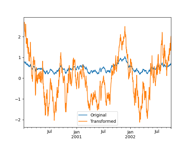
若变换函数返回较低维度的结果,该结果会广播到输入数组的形状。
In [142]: ts.groupby(lambda x: x.year).transform(lambda x: x.max() - x.min())
Out[142]:
2000-01-08    0.623893
2000-01-09    0.623893
2000-01-10    0.623893
2000-01-11    0.623893
2000-01-12    0.623893
                ...
2002-09-30    0.558275
2002-10-01    0.558275
2002-10-02    0.558275
2002-10-03    0.558275
2002-10-04    0.558275
Freq: D, Length: 1001, dtype: float64
另一种常见变换是用组均值替换缺失数据。
In [143]: cols = ["A", "B", "C"]

In [144]: values = np.random.randn(1000, 3)

In [145]: values[np.random.randint(0, 1000, 100), 0] = np.nan

In [146]: values[np.random.randint(0, 1000, 50), 1] = np.nan

In [147]: values[np.random.randint(0, 1000, 200), 2] = np.nan

In [148]: data_df = pd.DataFrame(values, columns=cols)

In [149]: data_df
Out[149]:
            A         B         C
0    1.539708 -1.166480  0.533026
1    1.302092 -0.505754       NaN
2   -0.371983  1.104803 -0.651520
3   -1.309622  1.118697 -1.161657
4   -1.924296  0.396437  0.812436
..        ...       ...       ...
995 -0.093110  0.683847 -0.774753
996 -0.185043  1.438572       NaN
997 -0.394469 -0.642343  0.011374
998 -1.174126  1.857148       NaN
999  0.234564  0.517098  0.393534

[1000 rows x 3 columns]
In [150]: countries = np.array(["US", "UK", "GR", "JP"])

In [151]: key = countries[np.random.randint(0, 4, 1000)]

In [152]: grouped = data_df.groupby(key)

# Non-NA count in each group
In [153]: grouped.count()
Out[153]:
      A    B    C
GR  209  217  189
JP  240  255  217
UK  216  231  193
US  239  250  217

In [154]: transformed = grouped.transform(lambda x: x.fillna(x.mean()))
可以验证,变换没有改变各组的均值,且变换后的数据不再包含缺失值。
In [155]: grouped_trans = transformed.groupby(key)

In [156]: grouped.mean()  # original group means
Out[156]:
           A         B         C
GR -0.098371 -0.015420  0.068053
JP  0.069025  0.023100 -0.077324
UK  0.034069 -0.052580 -0.116525
US  0.058664 -0.020399  0.028603
In [157]: grouped_trans.mean()  # transformation did not change group means
Out[157]:
           A         B         C
GR -0.098371 -0.015420  0.068053
JP  0.069025  0.023100 -0.077324
UK  0.034069 -0.052580 -0.116525
US  0.058664 -0.020399  0.028603

In [158]: grouped.count()  # original has some missing data points
Out[158]:
      A    B    C
GR  209  217  189
JP  240  255  217
UK  216  231  193
US  239  250  217
In [159]: grouped_trans.count()  # counts after transformation
Out[159]:
      A    B    C
GR  228  228  228
JP  267  267  267
UK  247  247  247
US  258  258  258

In [160]: grouped_trans.size()  # Verify non-NA count equals group size
Out[160]:
GR    228
JP    267
UK    247
US    258
dtype: int64
如前面的提示所述,本节所有示例都可以使用内置方法更高效地计算。下方代码把较慢的 UDF 写法注释掉,并在其后给出较快的替代方案。
# result = ts.groupby(lambda x: x.year).transform(
#     lambda x: (x - x.mean()) / x.std()
# )
In [161]: grouped = ts.groupby(lambda x: x.year)

In [162]: result = (ts - grouped.transform("mean")) / grouped.transform("std")
# result = ts.groupby(lambda x: x.year).transform(lambda x: x.max() - x.min())
In [163]: grouped = ts.groupby(lambda x: x.year)

In [164]: result = grouped.transform("max") - grouped.transform("min")

# grouped = data_df.groupby(key)
# result = grouped.transform(lambda x: x.fillna(x.mean()))
In [165]: grouped = data_df.groupby(key)

In [166]: result = data_df.fillna(grouped.transform("mean"))
窗口与重采样操作
可以直接对 GroupBy 调用 resample()、expanding() 和 rolling()。
下例按 A 列分组,再对 B 列的样本应用 rolling():
In [167]: df_re = pd.DataFrame({"A": [1] * 10 + [5] * 10, "B": np.arange(20)})

In [168]: df_re
Out[168]:
    A   B
0   1   0
1   1   1
2   1   2
3   1   3
4   1   4
.. ..  ..
15  5  15
16  5  16
17  5  17
18  5  18
19  5  19

[20 rows x 2 columns]

In [169]: df_re.groupby("A").rolling(4).B.mean()
Out[169]:
A
1  0      NaN
   1      NaN
   2      NaN
   3      1.5
   4      2.5
         ...
5  15    13.5
   16    14.5
   17    15.5
   18    16.5
   19    17.5
Name: B, Length: 20, dtype: float64
expanding() 会对每个组逐步扩大的范围执行指定操作;下例使用 sum():
In [170]: df_re.groupby("A").expanding().sum()
Out[170]:
          B
A
1 0     0.0
  1     1.0
  2     3.0
  3     6.0
  4    10.0
...     ...
5 15   75.0
  16   91.0
  17  108.0
  18  126.0
  19  145.0

[20 rows x 1 columns]
假设要对 DataFrame 的每一组调用 resample(),得到日频数据,再用 ffill() 填补缺失值:
In [171]: df_re = pd.DataFrame(
   .....:     {
   .....:         "date": pd.date_range(start="2016-01-01", periods=4, freq="W"),
   .....:         "group": [1, 1, 2, 2],
   .....:         "val": [5, 6, 7, 8],
   .....:     }
   .....: ).set_index("date")
   .....:

In [172]: df_re
Out[172]:
            group  val
date
2016-01-03      1    5
2016-01-10      1    6
2016-01-17      2    7
2016-01-24      2    8

In [173]: df_re.groupby("group").resample("1D").ffill()
Out[173]:
                  val
group date
1     2016-01-03    5
      2016-01-04    5
      2016-01-05    5
      2016-01-06    5
      2016-01-07    5
...               ...
2     2016-01-20    7
      2016-01-21    7
      2016-01-22    7
      2016-01-23    7
      2016-01-24    8

[16 rows x 1 columns]
筛选
筛选是从原分组对象中取出子集的 GroupBy 操作,可以删除整组、删除组内部分行,或者兼而有之。它返回调用对象筛选后的版本;若选择的列包含分组列,这些列也会保留。下例结果中包含 class。
In [174]: speeds
Out[174]:
          class           order  max_speed
falcon     bird   Falconiformes      389.0
parrot     bird  Psittaciformes       24.0
lion     mammal       Carnivora       80.2
monkey   mammal        Primates        NaN
leopard  mammal       Carnivora       58.0

In [175]: speeds.groupby("class").nth(1)
Out[175]:
         class           order  max_speed
parrot    bird  Psittaciformes       24.0
monkey mammal Primates NaN筛选会遵循对 GroupBy 对象所作的选列操作。
In [176]: speeds.groupby("class")[["order", "max_speed"]].nth(1)
Out[176]:
                 order  max_speed
parrot  Psittaciformes       24.0
monkey        Primates        NaN
内置筛选方法
以下 GroupBy 方法执行筛选,且都有高效的 GroupBy 专用实现。
| 方法 | 说明 |
|---|---|
head() |
选择每组开头的一行或多行 |
nth() |
选择每组第 n 行或指定的多行 |
tail() |
选择每组末尾的一行或多行 |
也可以结合变换与布尔索引,实现复杂的组内筛选。例如,每组包含若干产品及其数量,现在希望保留数量最大的产品,且累计数量不超过该组总量的 90%。
In [177]: product_volumes = pd.DataFrame(
   .....:     {
   .....:         "group": list("xxxxyyy"),
   .....:         "product": list("abcdefg"),
   .....:         "volume": [10, 30, 20, 15, 40, 10, 20],
   .....:     }
   .....: )
   .....:

In [178]: product_volumes
Out[178]:
  group product  volume
0     x       a      10
1     x       b      30
2     x       c      20
3     x       d      15
4     y       e      40
5     y       f      10
6     y       g      20

# Sort by volume to select the largest products first
In [179]: product_volumes = product_volumes.sort_values("volume", ascending=False)

In [180]: grouped = product_volumes.groupby("group")["volume"]

In [181]: cumpct = grouped.cumsum() / grouped.transform("sum")

In [182]: cumpct
Out[182]:
4    0.571429
1    0.400000
2    0.666667
6    0.857143
3    0.866667
0    1.000000
5    1.000000
Name: volume, dtype: float64

In [183]: significant_products = product_volumes[cumpct <= 0.9]
In [184]: significant_products.sort_values(["group", "product"])
Out[184]:
  group product  volume
1     x       b      30
2     x       c      20
3     x       d      15
4     y       e      40
6     y       g      20
filter 方法
filter 接受一个用户定义函数。该函数对整个组求值,并返回 True 或 False;filter 最终保留函数返回 True 的那些组。
假设只希望保留组内总和大于 2 的组中的元素:
In [185]: sf = pd.Series([1, 1, 2, 3, 3, 3])

In [186]: sf.groupby(sf).filter(lambda x: x.sum() > 2)
Out[186]:
3    3
4    3
5    3
dtype: int64
另一个有用操作,是删除成员数量过少的组中的元素。
In [187]: dff = pd.DataFrame({"A": np.arange(8), "B": list("aabbbbcc")})

In [188]: dff.groupby("B").filter(lambda x: len(x) > 2)
Out[188]:
   A  B
2  2  b
3  3  b
4  4  b
5  5  b
也可以不删除未通过筛选的组,而是返回与输入具有相同索引的对象,把未通过的组填为 NaN。
In [189]: dff.groupby("B").filter(lambda x: len(x) > 2, dropna=False)
Out[189]:
     A    B
0  NaN  NaN
1  NaN  NaN
2  2.0    b
3  3.0    b
4  4.0    b
5  5.0    b
6  NaN  NaN
7  NaN  NaN
对于多列 DataFrame,筛选函数应明确指定用哪一列作为判断依据。
In [190]: dff["C"] = np.arange(8)

In [191]: dff.groupby("B").filter(lambda x: len(x["C"]) > 2)
Out[191]:
   A  B  C
2  2  b  2
3  3  b  3
4  4  b  4
5  5  b  5
灵活的 apply
有些分组操作不属于聚合、变换或筛选。这时可以使用 apply 函数。
In [192]: df
Out[192]:
     A      B         C         D
0  foo    one -0.575247  1.346061
1  bar    one  0.254161  1.511763
2  foo    two -1.143704  1.627081
3  bar  three  0.215897 -0.990582
4  foo    two  1.193555 -0.441652
5  bar    two -0.077118  1.211526
6  foo    one -0.408530  0.268520
7  foo  three -0.862495  0.024580
In [193]: grouped = df.groupby("A")

# could also just call .describe()
In [194]: grouped["C"].apply(lambda x: x.describe())
Out[194]:
A
bar  count    3.000000
     mean     0.130980
     std      0.181231
     min     -0.077118
     25%      0.069390
                ...
foo  min     -1.143704
     25%     -0.862495
     50%     -0.575247
     75%     -0.408530
     max      1.193555
Name: C, Length: 16, dtype: float64
返回结果的维度也可能改变:
In [195]: grouped = df.groupby('A')['C']

In [196]: def f(group):
   .....:     return pd.DataFrame({'original': group,
   .....:                          'demeaned': group - group.mean()})
   .....:

In [197]: grouped.apply(f)
Out[197]:
       original  demeaned
A
bar 1  0.254161  0.123181
    3  0.215897  0.084917
    5 -0.077118 -0.208098
foo 0 -0.575247 -0.215962
    2 -1.143704 -0.784420
    4  1.193555  1.552839
    6 -0.408530 -0.049245
    7 -0.862495 -0.503211
对 Series 使用 apply 时,被调用函数的返回值本身也可以是 Series;结果可能被提升为 DataFrame:
In [198]: def f(x):
   .....:     return pd.Series([x, x ** 2], index=["x", "x^2"])
   .....:

In [199]: s = pd.Series(np.random.rand(5))

In [200]: s
Out[200]:
0    0.582898
1    0.098352
2    0.001438
3    0.009420
4    0.815826
dtype: float64

In [201]: s.apply(f)
Out[201]:
          x       x^2
0  0.582898  0.339770
1  0.098352  0.009673
2  0.001438  0.000002
3  0.009420  0.000089
4  0.815826  0.665572
与 aggregate() 方法 类似,结果类型由 apply 函数决定。若不同组返回不同类型,pandas 会按照构造 DataFrame 的规则确定共同类型。
用 group_keys 控制分组列的位置
使用默认值为 True 的 group_keys 参数,可以控制是否把分组列加入索引。比较以下两种结果:
In [202]: df.groupby("A", group_keys=True).apply(lambda x: x)
Out[202]:
           B         C         D
A
bar 1    one  0.254161  1.511763
    3  three  0.215897 -0.990582
    5    two -0.077118  1.211526
foo 0    one -0.575247  1.346061
    2    two -1.143704  1.627081
    4    two  1.193555 -0.441652
    6    one -0.408530  0.268520
    7  three -0.862495  0.024580
与:
In [203]: df.groupby("A", group_keys=False).apply(lambda x: x)
Out[203]:
       B         C         D
0    one -0.575247  1.346061
1    one  0.254161  1.511763
2    two -1.143704  1.627081
3  three  0.215897 -0.990582
4    two  1.193555 -0.441652
5    two -0.077118  1.211526
6    one -0.408530  0.268520
7  three -0.862495  0.024580
Numba 加速
安装可选依赖 Numba 后,transform 和 aggregate 支持 engine='numba' 与 engine_kwargs 参数。参数用法和性能注意事项见 通过 Numba 提升性能。
函数签名必须准确地以 values, index 开头:每组的数据会传入 values,该组的索引会传入 index。
其他实用功能
排除非数值列
再次考虑前面使用的 DataFrame:
In [204]: df
Out[204]:
     A      B         C         D
0  foo    one -0.575247  1.346061
1  bar    one  0.254161  1.511763
2  foo    two -1.143704  1.627081
3  bar  three  0.215897 -0.990582
4  foo    two  1.193555 -0.441652
5  bar    two -0.077118  1.211526
6  foo    one -0.408530  0.268520
7  foo  three -0.862495  0.024580
假设希望按 A 列分组计算标准差。B 列不是数值数据,我们并不关心它;可指定 numeric_only=True,排除非数值列:
In [205]: df.groupby("A").std(numeric_only=True)
Out[205]:
            C         D
A
bar  0.181231  1.366330
foo  0.912265  0.884785
df.groupby('A').colname.std() 比 df.groupby('A').std().colname 更高效。因此,如果只需要某一列的聚合结果,可以先选取该列,再执行聚合。
In [206]: from decimal import Decimal

In [207]: df_dec = pd.DataFrame(
   .....:     {
   .....:         "id": [1, 2, 1, 2],
   .....:         "int_column": [1, 2, 3, 4],
   .....:         "dec_column": [
   .....:             Decimal("0.50"),
   .....:             Decimal("0.15"),
   .....:             Decimal("0.25"),
   .....:             Decimal("0.40"),
   .....:         ],
   .....:     }
   .....: )
   .....:

In [208]: df_dec.groupby(["id"])[["dec_column"]].sum()
Out[208]:
   dec_column
id
1        0.75
2        0.55
处理已出现与未出现的分类值
使用 Categorical 作为单个分组器或多个分组器中的一个时,observed 控制返回全部可能分类值的笛卡尔积(observed=False),还是只返回实际出现的组合(observed=True)。
显示全部分类值:
In [209]: pd.Series([1, 1, 1]).groupby(
   .....:     pd.Categorical(["a", "a", "a"], categories=["a", "b"]), observed=False
   .....: ).count()
   .....:
Out[209]:
a    3
b    0
dtype: int64
只显示实际出现的分类值:
In [210]: pd.Series([1, 1, 1]).groupby(
   .....:     pd.Categorical(["a", "a", "a"], categories=["a", "b"]), observed=True
   .....: ).count()
   .....:
Out[210]:
a    3
dtype: int64
返回分组结果的数据类型始终包含参与分组的全部分类类别。
In [211]: s = (
   .....:     pd.Series([1, 1, 1])
   .....:     .groupby(pd.Categorical(["a", "a", "a"], categories=["a", "b"]), observed=True)
   .....:     .count()
   .....: )
   .....:

In [212]: s.index.dtype
Out[212]: CategoricalDtype(categories=['a', 'b'], ordered=False, categories_dtype=str)
NA 分组的处理
这里的 NA 泛指任何缺失值,包括 NA、NaN、NaT 和 None。分组键中出现的缺失值默认会被排除,也就是丢弃“NA 组”。指定 dropna=False 可将它们保留。
In [213]: df = pd.DataFrame({"key": [1.0, 1.0, np.nan, 2.0, np.nan], "A": [1, 2, 3, 4, 5]})

In [214]: df
Out[214]:
   key  A
0  1.0  1
1  1.0  2
2  NaN  3
3  2.0  4
4  NaN  5
In [215]: df.groupby("key", dropna=True).sum()
Out[215]:
     A
key
1.0  3
2.0  4

In [216]: df.groupby("key", dropna=False).sum()
Out[216]:
     A
key
1.0  3
2.0  4
NaN  8
按有序分类分组
pandas 的 Categorical 实例可以用作组键,并保留分类层级的顺序。在 observed=False 且 sort=False 时,未出现的类别会按其分类顺序放在结果末尾。
In [217]: days = pd.Categorical(
   .....:     values=["Wed", "Mon", "Thu", "Mon", "Wed", "Sat"],
   .....:     categories=["Mon", "Tue", "Wed", "Thu", "Fri", "Sat", "Sun"],
   .....: )
   .....:
In [218]: data = pd.DataFrame(
   .....:    {
   .....:        "day": days,
   .....:        "workers": [3, 4, 1, 4, 2, 2],
   .....:    }
   .....: )
   .....:

In [219]: data
Out[219]:
   day  workers
0  Wed        3
1  Mon        4
2  Thu        1
3  Mon        4
4  Wed        2
5  Sat        2

In [220]: data.groupby("day", observed=False, sort=True).sum()
Out[220]:
     workers
day
Mon        8
Tue        0
Wed        5
Thu        1
Fri        0
Sat        2
Sun        0

In [221]: data.groupby("day", observed=False, sort=False).sum()
Out[221]:
     workers
day
Wed        5
Mon        8
Thu        1
Sat        2
Tue        0
Fri        0
Sun        0
使用 Grouper 指定分组规则
有时需要提供更多信息才能正确分组,可以使用 pd.Grouper 对具体分组规则进行控制。
In [222]: import datetime

In [223]: df = pd.DataFrame(
   .....:     {
   .....:         "Branch": "A A A A A A A B".split(),
   .....:         "Buyer": "Carl Mark Carl Carl Joe Joe Joe Carl".split(),
   .....:         "Quantity": [1, 3, 5, 1, 8, 1, 9, 3],
   .....:         "Date": [
   .....:             datetime.datetime(2013, 1, 1, 13, 0),
   .....:             datetime.datetime(2013, 1, 1, 13, 5),
   .....:             datetime.datetime(2013, 10, 1, 20, 0),
   .....:             datetime.datetime(2013, 10, 2, 10, 0),
   .....:             datetime.datetime(2013, 10, 1, 20, 0),
   .....:             datetime.datetime(2013, 10, 2, 10, 0),
   .....:             datetime.datetime(2013, 12, 2, 12, 0),
   .....:             datetime.datetime(2013, 12, 2, 14, 0),
   .....:         ],
   .....:     }
   .....: )
   .....:

In [224]: df
Out[224]:
  Branch Buyer  Quantity                Date
0      A  Carl         1 2013-01-01 13:00:00
1      A  Mark         3 2013-01-01 13:05:00
2      A  Carl         5 2013-10-01 20:00:00
3      A  Carl         1 2013-10-02 10:00:00
4      A   Joe         8 2013-10-01 20:00:00
5      A   Joe         1 2013-10-02 10:00:00
6      A   Joe         9 2013-12-02 12:00:00
7      B  Carl         3 2013-12-02 14:00:00
按某一列以指定频率分组,类似于重采样。
In [225]: df.groupby([pd.Grouper(freq="1ME", key="Date"), "Buyer"])[["Quantity"]].sum()
Out[225]:
                  Quantity
Date       Buyer
2013-01-31 Carl          1
           Mark          3
2013-10-31 Carl          6
           Joe           9
2013-12-31 Carl          3
           Joe           9
指定 freq 时,pd.Grouper 返回 pandas.api.typing.TimeGrouper 实例。如果某列与索引同名,可用 key 指定按列分组,用 level 指定按索引分组。
In [226]: df = df.set_index("Date")

In [227]: df["Date"] = df.index + pd.offsets.MonthEnd(2)

In [228]: df.groupby([pd.Grouper(freq="6ME", key="Date"), "Buyer"])[["Quantity"]].sum()
Out[228]:
                  Quantity
Date       Buyer
2013-02-28 Carl          1
           Mark          3
2014-02-28 Carl          9
           Joe          18

In [229]: df.groupby([pd.Grouper(freq="6ME", level="Date"), "Buyer"])[["Quantity"]].sum()
Out[229]:
                  Quantity
Date       Buyer
2013-01-31 Carl          1
           Mark          3
2014-01-31 Carl          9
           Joe          18
取每组的前几行
与 DataFrame 和 Series 一样,可以对 GroupBy 调用 head 与 tail:
In [230]: df = pd.DataFrame([[1, 2], [1, 4], [5, 6]], columns=["A", "B"])

In [231]: df
Out[231]:
   A  B
0  1  2
1  1  4
2  5  6

In [232]: g = df.groupby("A")

In [233]: g.head(1)
Out[233]:
   A  B
0  1  2
2  5  6

In [234]: g.tail(1)
Out[234]:
   A  B
1  1  4
2  5  6
这些方法返回每组最前面或最后面的 n 行。
取每组第 n 行
使用 DataFrameGroupBy.nth() 或 SeriesGroupBy.nth() 选择每组第 n 项。参数可以是整数、整数列表、切片或切片列表,示例见下文。如果某组不存在第 n 项,不会报错,只是不返回该组对应的行。
一般来说,此操作属于筛选。某些情况下它恰好每组返回一行,也具有归约的效果;但因为通常可能每组返回零行或多行,pandas 始终将其视为筛选。
In [235]: df = pd.DataFrame([[1, np.nan], [1, 4], [5, 6]], columns=["A", "B"])

In [236]: g = df.groupby("A")

In [237]: g.nth(0)
Out[237]:
   A    B
0  1  NaN
2  5  6.0

In [238]: g.nth(-1)
Out[238]:
   A    B
1  1  4.0
2  5  6.0

In [239]: g.nth(1)
Out[239]:
   A    B
1  1  4.0
如果某组不存在第 n 项,结果就不包含相应行。特别是,当 n 大于所有组的大小时,会返回空 DataFrame。
In [240]: g.nth(5)
Out[240]:
Empty DataFrame
Columns: [A, B]
Index: []
如果希望选择第 n 个非缺失项,可使用 dropna 参数。对于 DataFrame,与调用 dropna 一样,参数应为 'any' 或 'all':
# nth(0) is the same as g.first()
In [241]: g.nth(0, dropna="any")
Out[241]:
   A    B
1  1  4.0
2  5  6.0

In [242]: g.first()
Out[242]:
     B
A
1  4.0
5  6.0

# nth(-1) is the same as g.last()
In [243]: g.nth(-1, dropna="any")
Out[243]:
   A    B
1  1  4.0
2  5  6.0

In [244]: g.last()
Out[244]:
     B
A
1  4.0
5  6.0

In [245]: g.B.nth(0, dropna="all")
Out[245]:
1    4.0
2    6.0
Name: B, dtype: float64
还可以用整数列表指定多个 n 值,从每组选择多行。
In [246]: business_dates = pd.date_range(start="4/1/2014", end="6/30/2014", freq="B")

In [247]: df = pd.DataFrame(1, index=business_dates, columns=["a", "b"])

# get the first, 4th, and last date index for each month
In [248]: df.groupby([df.index.year, df.index.month]).nth([0, 3, -1])
Out[248]:
            a  b
2014-04-01  1  1
2014-04-04  1  1
2014-04-30  1  1
2014-05-01  1  1
2014-05-06  1  1
2014-05-30  1  1
2014-06-02  1  1
2014-06-05  1  1
2014-06-30  1  1
也可以使用切片或切片列表。
In [249]: df.groupby([df.index.year, df.index.month]).nth[1:]
Out[249]:
            a  b
2014-04-02  1  1
2014-04-03  1  1
2014-04-04  1  1
2014-04-07  1  1
2014-04-08  1  1
...        .. ..
2014-06-24  1  1
2014-06-25  1  1
2014-06-26  1  1
2014-06-27  1  1
2014-06-30  1  1

[62 rows x 2 columns]

In [250]: df.groupby([df.index.year, df.index.month]).nth[1:, :-1]
Out[250]:
            a  b
2014-04-01  1  1
2014-04-02  1  1
2014-04-03  1  1
2014-04-04  1  1
2014-04-07  1  1
...        .. ..
2014-06-24  1  1
2014-06-25  1  1
2014-06-26  1  1
2014-06-27  1  1
2014-06-30  1  1

[65 rows x 2 columns]
给组内元素编号
使用 cumcount 可查看每行在所属组内的出现次序:
In [251]: dfg = pd.DataFrame(list("aaabba"), columns=["A"])

In [252]: dfg
Out[252]:
   A
0  a
1  a
2  a
3  b
4  b
5  a

In [253]: dfg.groupby("A").cumcount()
Out[253]:
0    0
1    1
2    2
3    0
4    1
5    3
dtype: int64

In [254]: dfg.groupby("A").cumcount(ascending=False)
Out[254]:
0    3
1    2
2    1
3    1
4    0
5    0
dtype: int64
给组编号
使用 DataFrameGroupBy.ngroup() 可查看组的顺序;这与 cumcount 返回的组内行顺序不同。
组的编号对应遍历 GroupBy 对象时看到各组的顺序,并非组在数据中首次出现的顺序。
In [255]: dfg = pd.DataFrame(list("aaabba"), columns=["A"])

In [256]: dfg
Out[256]:
   A
0  a
1  a
2  a
3  b
4  b
5  a

In [257]: dfg.groupby("A").ngroup()
Out[257]:
0    0
1    0
2    0
3    1
4    1
5    0
dtype: int64
In [258]: dfg.groupby("A").ngroup(ascending=False)
Out[258]:
0    1
1    1
2    1
3    0
4    0
5    1
dtype: int64
绘图
GroupBy 也支持某些绘图方法。假设我们怀疑第 1 列在 B 组中的平均值约为其他组的 3 倍:
In [259]: np.random.seed(1234)

In [260]: df = pd.DataFrame(np.random.randn(50, 2))

In [261]: df["g"] = np.random.choice(["A", "B"], size=50)

In [262]: df.loc[df["g"] == "B", 1] += 3
可以很方便地用箱线图呈现:
In [263]: df.groupby("g").boxplot()
Out[263]:
A         Axes(0.1,0.15;0.363636x0.75)
B    Axes(0.536364,0.15;0.363636x0.75)
dtype: object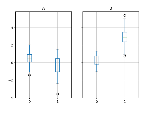
调用 boxplot 返回一个字典,其键为分组列 g 的值 A 和 B。可用 boxplot 的 return_type 参数控制字典中的值;详见 可视化文档。
通过管道串联函数调用
与 DataFrame 和 Series 的 pipe 类似,接受 GroupBy 对象的函数也可以用 pipe 串联,使代码更清晰易读。.pipe 的一般介绍见 此处。
需要复用 GroupBy 对象时,组合 .groupby 与 .pipe 往往很有用。
例如,一个 DataFrame 包含门店、产品、销售收入和销量。我们希望按门店与产品分组,计算单价,即收入除以销量。可以分多步完成,但管道写法可能更易读。先准备数据:
In [264]: n = 1000

In [265]: df = pd.DataFrame(
   .....:     {
   .....:         "Store": np.random.choice(["Store_1", "Store_2"], n),
   .....:         "Product": np.random.choice(["Product_1", "Product_2"], n),
   .....:         "Revenue": (np.random.random(n) * 50 + 10).round(2),
   .....:         "Quantity": np.random.randint(1, 10, size=n),
   .....:     }
   .....: )
   .....:

In [266]: df.head(2)
Out[266]:
     Store    Product  Revenue  Quantity
0  Store_2  Product_1    26.12         1
1  Store_2  Product_1    28.86         1
现在计算每个门店、每种产品的单价。
In [267]: (
   .....:     df.groupby(["Store", "Product"])
   .....:     .pipe(lambda grp: grp.Revenue.sum() / grp.Quantity.sum())
   .....:     .unstack()
   .....:     .round(2)
   .....: )
   .....:
Out[267]:
Product  Product_1  Product_2
Store
Store_1       6.82       7.05
Store_2       6.30       6.64
如果要把分组对象传给任意函数,管道也能清楚地表达意图,例如:
In [268]: def mean(groupby):
   .....:     return groupby.mean()
   .....:

In [269]: df.groupby(["Store", "Product"]).pipe(mean)
Out[269]:
                     Revenue  Quantity
Store   Product
Store_1 Product_1  34.622727  5.075758
        Product_2  35.482815  5.029630
Store_2 Product_1  32.972837  5.237589
        Product_2  34.684360  5.224000
这里 mean 接收 GroupBy 对象,并为每个门店与产品组合分别计算 Revenue 和 Quantity 的均值。它可以是任何接受 GroupBy 对象的函数;.pipe 会将 GroupBy 对象作为参数传入指定函数。
示例
多列因子化编码
使用 DataFrameGroupBy.ngroup(),可以类似 factorize() 那样提取分组信息,详见 重塑 API。这种方式自然适用于来自不同来源、具有不同数据类型的多列。当组内行之间的关系比具体内容更重要时,可以把它作为处理中间的分类编码步骤,也可作为只接受整数编码的算法的输入。
关于 pandas 完整分类数据支持,参阅 分类数据介绍 和 API 文档。
In [270]: dfg = pd.DataFrame({"A": [1, 1, 2, 3, 2], "B": list("aaaba")})

In [271]: dfg
Out[271]:
   A  B
0  1  a
1  1  a
2  2  a
3  3  b
4  2  a

In [272]: dfg.groupby(["A", "B"]).ngroup()
Out[272]:
0    0
1    0
2    1
3    2
4    1
dtype: int64

In [273]: dfg.groupby(["A", [0, 0, 0, 1, 1]]).ngroup()
Out[273]:
0    0
1    0
2    1
3    3
4    2
dtype: int64
通过索引分组实现“重采样”
重采样是根据已有观测数据,或根据生成数据的模型,生成新的假设样本。新样本与原有样本相似。
对于非日期时间类索引,可以采用以下方式实现重采样。
下例中的 df.index // 5 返回整数数组,用来确定 groupby 操作的分组选择。
In [274]: df = pd.DataFrame(np.random.randn(10, 2))

In [275]: df
Out[275]:
          0         1
0 -0.793893  0.321153
1  0.342250  1.618906
2 -0.975807  1.918201
3 -0.810847 -1.405919
4 -1.977759  0.461659
5  0.730057 -1.316938
6 -0.751328  0.528290
7 -0.257759 -1.081009
8  0.505895 -1.701948
9 -1.006349  0.020208

In [276]: df.index // 5
Out[276]: Index([0, 0, 0, 0, 0, 1, 1, 1, 1, 1], dtype='int64')

In [277]: df.groupby(df.index // 5).std()
Out[277]:
          0         1
0  0.823647  1.312912
1  0.760109  0.942941
返回 Series 以传递名称
对 DataFrame 的列分组,计算一组指标,再返回带名称的 Series。Series 的名称会成为列索引名称。这在结合堆叠等重塑操作时尤其有用,因为列索引名称会成为插入列的名称:
In [278]: df = pd.DataFrame(
   .....:     {
   .....:         "a": [0, 0, 0, 0, 1, 1, 1, 1, 2, 2, 2, 2],
   .....:         "b": [0, 0, 1, 1, 0, 0, 1, 1, 0, 0, 1, 1],
   .....:         "c": [1, 0, 1, 0, 1, 0, 1, 0, 1, 0, 1, 0],
   .....:         "d": [0, 0, 0, 1, 0, 0, 0, 1, 0, 0, 0, 1],
   .....:     }
   .....: )
   .....:

In [279]: def compute_metrics(x):
   .....:     result = {"b_sum": x["b"].sum(), "c_mean": x["c"].mean()}
   .....:     return pd.Series(result, name="metrics")
   .....:

In [280]: result = df.groupby("a").apply(compute_metrics)

In [281]: result
Out[281]:
metrics  b_sum  c_mean
a
0          2.0     0.5
1          2.0     0.5
2          2.0     0.5

In [282]: result.stack()
Out[282]:
a  metrics
0  b_sum      2.0
   c_mean     0.5
1  b_sum      2.0
   c_mean     0.5
2  b_sum      2.0
   c_mean     0.5
dtype: float64










暂无评论内容