PyTorch 知识蒸馏教程

原文创建于 2023 年 8 月 22 日，最后更新于 2025 年 1 月 24 日，标注的最后验证日期为 2024 年 11 月 5 日。

作者：Alexandros Chariton。

知识蒸馏把大型、计算成本较高的模型所学到的知识传递给小模型，以期保留有效的预测能力。这有助于在算力较弱的硬件上部署，并让推理更快、更高效。

本教程通过一系列实验，以较强的网络作为教师，提高轻量网络的分类准确率。基本思路是在训练中改变学生的权重，让部署时仍使用轻量网络，应用场景包括无人机和手机。所需操作都由 torch 和 torchvision 提供，无需其他第三方包。

这里的推理成本不增加，是指部署时只保留学生用于分类的分支。后面的回归器示例仍会在 forward 中执行辅助分支；若原样部署，就不能声称没有额外计算，需先移除仅供蒸馏训练使用的分支。

本教程将介绍：

• 修改模型类，提取隐藏表示并用于后续计算。

• 修改 PyTorch 的常规训练循环，在分类交叉熵等主要损失之外加入额外损失。

• 用复杂模型作为教师，改善轻量模型的表现。

前置条件

• 原文列出的硬件条件为一块 GPU、4 GB 显存。

• 原文列出 PyTorch v2.0 或更高版本。当前页面代码使用 torch.accelerator，实际运行时还需要所安装的 PyTorch 版本支持这一 API，不能仅凭旧的最低版本说明判断可用。

• CIFAR-10 数据集，由示例脚本下载。原文前置条件写作 /data，下面实际代码使用相对目录 ./data。本译稿保留代码路径。以下设备信息、下载进度、训练损失和准确率均来自原文输出，不是本机执行结果。

import torch
import torch.nn as nn
import torch.optim as optim
import torchvision.transforms as transforms
import torchvision.datasets as datasets

# Check if the current `accelerator <https://pytorch.org/docs/stable/torch.html#accelerators>`__
# is available, and if not, use the CPU
device = torch.accelerator.current_accelerator().type if torch.accelerator.is_available() else "cpu"
print(f"Using {device} device")

Using cuda device

加载 CIFAR-10

CIFAR-10 是一个包含十个类别的常用图片数据集。目标是为每张输入图片预测其中一个类别。

CIFAR-10 十类图片示例

图：CIFAR-10 图片示例。

输入图片是 RGB 图像，有三个通道，尺寸为 32×32 像素。因此，每张图片由 3×32×32＝3072 个取值在 0 至 255 之间的数描述。神经网络通常会归一化输入，以避免常用激活函数饱和，并提高数值稳定性。这里的处理是逐通道减去均值、再除以标准差。

代码使用 mean=[0.485, 0.456, 0.406] 和 std=[0.229, 0.224, 0.225]。原文把这组数描述为 CIFAR-10 训练子集的统计量；这个来源说明不准确。这组数也用于 torchvision 的 ImageNet 预训练模型预处理，本例应理解为采用这组预设常数，而非已经在此计算了 CIFAR-10 的统计量。

测试集仍使用与训练集相同的常数，而不重新估计均值与标准差，因为网络是在上述处理得到的特征上训练的，测试时需要保持一致。在实际应用的设定中，训练阶段也不应依赖尚不可访问的测试数据来估计预处理参数。

通常会把调参过程中保留的数据称为验证集。根据验证集优化模型后，再用另一份独立的测试集作最终评估，避免对单一指标反复贪心优化，造成模型选择偏差。

# Below we are preprocessing data for CIFAR-10. We use an arbitrary batch size of 128.
transforms_cifar = transforms.Compose([
    transforms.ToTensor(),
    transforms.Normalize(mean=[0.485, 0.456, 0.406], std=[0.229, 0.224, 0.225]),
])

# Loading the CIFAR-10 dataset:
train_dataset = datasets.CIFAR10(root='./data', train=True, download=True, transform=transforms_cifar)
test_dataset = datasets.CIFAR10(root='./data', train=False, download=True, transform=transforms_cifar)

  0%|          | 0.00/170M [00:00<?, ?B/s]
  0%|          | 164k/170M [00:00<01:45, 1.62MB/s]
  0%|          | 590k/170M [00:00<00:55, 3.06MB/s]
  1%|          | 983k/170M [00:00<00:50, 3.35MB/s]
  1%|          | 1.38M/170M [00:00<00:47, 3.52MB/s]
  1%|          | 1.74M/170M [00:00<00:47, 3.55MB/s]
  1%|          | 2.10M/170M [00:00<00:50, 3.35MB/s]
  1%|▏         | 2.46M/170M [00:00<00:51, 3.24MB/s]
  2%|▏         | 2.82M/170M [00:00<00:50, 3.31MB/s]
  2%|▏         | 3.34M/170M [00:00<00:44, 3.78MB/s]
  2%|▏         | 4.10M/170M [00:01<00:34, 4.87MB/s]
  3%|▎         | 4.62M/170M [00:01<00:34, 4.76MB/s]
  3%|▎         | 5.11M/170M [00:01<00:36, 4.58MB/s]
  3%|▎         | 5.60M/170M [00:01<00:37, 4.44MB/s]
  4%|▎         | 6.06M/170M [00:01<00:37, 4.38MB/s]
  4%|▍         | 6.52M/170M [00:01<00:38, 4.31MB/s]
  4%|▍         | 6.98M/170M [00:01<00:38, 4.27MB/s]
  4%|▍         | 7.44M/170M [00:01<00:38, 4.23MB/s]
  5%|▍         | 7.86M/170M [00:01<00:38, 4.17MB/s]
  5%|▍         | 8.29M/170M [00:02<00:39, 4.16MB/s]
  5%|▌         | 8.72M/170M [00:02<00:39, 4.14MB/s]
  5%|▌         | 9.14M/170M [00:02<00:39, 4.12MB/s]
  6%|▌         | 9.57M/170M [00:02<00:39, 4.10MB/s]
  6%|▌         | 9.99M/170M [00:02<00:39, 4.10MB/s]
  6%|▌         | 10.4M/170M [00:02<00:38, 4.11MB/s]
  6%|▋         | 10.8M/170M [00:02<00:38, 4.10MB/s]
  7%|▋         | 11.3M/170M [00:02<00:39, 4.03MB/s]
  7%|▋         | 11.7M/170M [00:02<00:39, 4.01MB/s]
  7%|▋         | 12.1M/170M [00:03<00:39, 3.98MB/s]
  7%|▋         | 12.6M/170M [00:03<00:39, 3.97MB/s]
  8%|▊         | 13.0M/170M [00:03<00:40, 3.93MB/s]
  8%|▊         | 13.4M/170M [00:03<00:40, 3.92MB/s]
  8%|▊         | 13.8M/170M [00:03<00:39, 3.93MB/s]
  8%|▊         | 14.2M/170M [00:03<00:39, 3.93MB/s]
  9%|▊         | 14.6M/170M [00:03<00:39, 3.92MB/s]
  9%|▉         | 15.0M/170M [00:03<00:39, 3.89MB/s]
  9%|▉         | 15.4M/170M [00:03<00:40, 3.83MB/s]
  9%|▉         | 15.8M/170M [00:03<00:40, 3.82MB/s]
  9%|▉         | 16.2M/170M [00:04<00:40, 3.81MB/s]
 10%|▉         | 16.5M/170M [00:04<00:40, 3.81MB/s]
 10%|▉         | 16.9M/170M [00:04<00:40, 3.80MB/s]
 10%|█         | 17.3M/170M [00:04<00:40, 3.81MB/s]
 10%|█         | 17.7M/170M [00:04<00:40, 3.80MB/s]
 11%|█         | 18.1M/170M [00:04<00:40, 3.77MB/s]
 11%|█         | 18.5M/170M [00:04<00:40, 3.75MB/s]
 11%|█         | 18.9M/170M [00:04<00:40, 3.74MB/s]
 11%|█▏        | 19.3M/170M [00:04<00:40, 3.71MB/s]
 12%|█▏        | 19.7M/170M [00:05<00:41, 3.66MB/s]
 12%|█▏        | 20.1M/170M [00:05<00:41, 3.66MB/s]
 12%|█▏        | 20.5M/170M [00:05<00:41, 3.64MB/s]
 12%|█▏        | 20.9M/170M [00:05<00:41, 3.61MB/s]
 12%|█▏        | 21.3M/170M [00:05<00:41, 3.62MB/s]
 13%|█▎        | 21.7M/170M [00:05<00:41, 3.62MB/s]
 13%|█▎        | 22.1M/170M [00:05<00:40, 3.62MB/s]
 13%|█▎        | 22.4M/170M [00:05<00:40, 3.63MB/s]
 13%|█▎        | 22.8M/170M [00:05<00:40, 3.61MB/s]
 14%|█▎        | 23.2M/170M [00:05<00:40, 3.66MB/s]
 14%|█▍        | 23.7M/170M [00:06<00:39, 3.75MB/s]
 14%|█▍        | 24.1M/170M [00:06<00:38, 3.80MB/s]
 14%|█▍        | 24.4M/170M [00:06<00:38, 3.83MB/s]
 15%|█▍        | 24.8M/170M [00:06<00:37, 3.84MB/s]
 15%|█▍        | 25.2M/170M [00:06<00:37, 3.86MB/s]
 15%|█▌        | 25.6M/170M [00:06<00:37, 3.84MB/s]
 15%|█▌        | 26.1M/170M [00:06<00:37, 3.88MB/s]
 16%|█▌        | 26.5M/170M [00:06<00:36, 3.90MB/s]
 16%|█▌        | 26.9M/170M [00:06<00:36, 3.91MB/s]
 16%|█▌        | 27.3M/170M [00:07<00:36, 3.94MB/s]
 16%|█▋        | 27.7M/170M [00:07<00:35, 3.97MB/s]
 17%|█▋        | 28.1M/170M [00:07<00:35, 4.00MB/s]
 17%|█▋        | 28.6M/170M [00:07<00:35, 4.02MB/s]
 17%|█▋        | 29.0M/170M [00:07<00:35, 4.03MB/s]
 17%|█▋        | 29.4M/170M [00:07<00:34, 4.04MB/s]
 18%|█▊        | 29.9M/170M [00:07<00:34, 4.07MB/s]
 18%|█▊        | 30.3M/170M [00:07<00:34, 4.10MB/s]
 18%|█▊        | 30.7M/170M [00:07<00:34, 4.08MB/s]
 18%|█▊        | 31.1M/170M [00:07<00:34, 4.07MB/s]
 19%|█▊        | 31.6M/170M [00:08<00:34, 4.08MB/s]
 19%|█▉        | 32.0M/170M [00:08<00:33, 4.10MB/s]
 19%|█▉        | 32.4M/170M [00:08<00:33, 4.09MB/s]
 19%|█▉        | 32.8M/170M [00:08<00:33, 4.14MB/s]
 20%|█▉        | 33.3M/170M [00:08<00:32, 4.24MB/s]
 20%|█▉        | 33.8M/170M [00:08<00:31, 4.31MB/s]
 20%|██        | 34.2M/170M [00:08<00:31, 4.33MB/s]
 20%|██        | 34.7M/170M [00:08<00:31, 4.37MB/s]
 21%|██        | 35.1M/170M [00:08<00:30, 4.40MB/s]
 21%|██        | 35.6M/170M [00:08<00:30, 4.39MB/s]
 21%|██        | 36.0M/170M [00:09<00:30, 4.34MB/s]
 21%|██▏       | 36.5M/170M [00:09<00:31, 4.31MB/s]
 22%|██▏       | 37.0M/170M [00:09<00:31, 4.25MB/s]
 22%|██▏       | 37.4M/170M [00:09<00:31, 4.24MB/s]
 22%|██▏       | 37.8M/170M [00:09<00:31, 4.24MB/s]
 22%|██▏       | 38.2M/170M [00:09<00:31, 4.21MB/s]
 23%|██▎       | 38.7M/170M [00:09<00:31, 4.22MB/s]
 23%|██▎       | 39.1M/170M [00:09<00:31, 4.24MB/s]
 23%|██▎       | 39.6M/170M [00:09<00:30, 4.24MB/s]
 23%|██▎       | 40.0M/170M [00:10<00:31, 4.21MB/s]
 24%|██▎       | 40.4M/170M [00:10<00:31, 4.19MB/s]
 24%|██▍       | 40.9M/170M [00:10<00:30, 4.19MB/s]
 24%|██▍       | 41.3M/170M [00:10<00:30, 4.18MB/s]
 24%|██▍       | 41.7M/170M [00:10<00:30, 4.16MB/s]
 25%|██▍       | 42.1M/170M [00:10<00:30, 4.16MB/s]
 25%|██▍       | 42.6M/170M [00:10<00:30, 4.15MB/s]
 25%|██▌       | 43.0M/170M [00:10<00:30, 4.16MB/s]
 25%|██▌       | 43.4M/170M [00:10<00:30, 4.13MB/s]
 26%|██▌       | 43.8M/170M [00:10<00:30, 4.11MB/s]
 26%|██▌       | 44.3M/170M [00:11<00:30, 4.07MB/s]
 26%|██▌       | 44.7M/170M [00:11<00:31, 4.05MB/s]
 26%|██▋       | 45.1M/170M [00:11<00:31, 3.99MB/s]
 27%|██▋       | 45.5M/170M [00:11<00:31, 3.98MB/s]
 27%|██▋       | 46.0M/170M [00:11<00:31, 3.98MB/s]
 27%|██▋       | 46.4M/170M [00:11<00:31, 3.96MB/s]
 27%|██▋       | 46.8M/170M [00:11<00:31, 3.94MB/s]
 28%|██▊       | 47.3M/170M [00:11<00:31, 3.94MB/s]
 28%|██▊       | 47.7M/170M [00:11<00:31, 3.92MB/s]
 28%|██▊       | 48.1M/170M [00:12<00:31, 3.90MB/s]
 28%|██▊       | 48.5M/170M [00:12<00:31, 3.88MB/s]
 29%|██▊       | 48.9M/170M [00:12<00:31, 3.84MB/s]
 29%|██▉       | 49.3M/170M [00:12<00:31, 3.84MB/s]
 29%|██▉       | 49.6M/170M [00:12<00:31, 3.84MB/s]
 29%|██▉       | 50.0M/170M [00:12<00:31, 3.83MB/s]
 30%|██▉       | 50.4M/170M [00:12<00:31, 3.84MB/s]
 30%|██▉       | 50.8M/170M [00:12<00:31, 3.84MB/s]
 30%|███       | 51.2M/170M [00:12<00:31, 3.81MB/s]
 30%|███       | 51.6M/170M [00:12<00:31, 3.79MB/s]
 31%|███       | 52.0M/170M [00:13<00:31, 3.77MB/s]
 31%|███       | 52.4M/170M [00:13<00:31, 3.77MB/s]
 31%|███       | 52.8M/170M [00:13<00:31, 3.78MB/s]
 31%|███       | 53.2M/170M [00:13<00:31, 3.77MB/s]
 31%|███▏      | 53.6M/170M [00:13<00:31, 3.76MB/s]
 32%|███▏      | 54.0M/170M [00:13<00:31, 3.74MB/s]
 32%|███▏      | 54.4M/170M [00:13<00:31, 3.73MB/s]
 32%|███▏      | 54.8M/170M [00:13<00:30, 3.74MB/s]
 32%|███▏      | 55.1M/170M [00:13<00:30, 3.74MB/s]
 33%|███▎      | 55.5M/170M [00:14<00:30, 3.75MB/s]
 33%|███▎      | 55.9M/170M [00:14<00:30, 3.79MB/s]
 33%|███▎      | 56.3M/170M [00:14<00:29, 3.81MB/s]
 33%|███▎      | 56.7M/170M [00:14<00:29, 3.84MB/s]
 33%|███▎      | 57.1M/170M [00:14<00:29, 3.86MB/s]
 34%|███▎      | 57.5M/170M [00:14<00:29, 3.86MB/s]
 34%|███▍      | 57.9M/170M [00:14<00:28, 3.90MB/s]
 34%|███▍      | 58.4M/170M [00:14<00:28, 3.92MB/s]
 34%|███▍      | 58.8M/170M [00:14<00:28, 3.91MB/s]
 35%|███▍      | 59.2M/170M [00:14<00:28, 3.92MB/s]
 35%|███▍      | 59.6M/170M [00:15<00:28, 3.92MB/s]
 35%|███▌      | 60.0M/170M [00:15<00:27, 3.96MB/s]
 35%|███▌      | 60.4M/170M [00:15<00:27, 3.98MB/s]
 36%|███▌      | 60.9M/170M [00:15<00:27, 4.02MB/s]
 36%|███▌      | 61.3M/170M [00:15<00:26, 4.05MB/s]
 36%|███▌      | 61.7M/170M [00:15<00:26, 4.06MB/s]
 36%|███▋      | 62.1M/170M [00:15<00:26, 4.06MB/s]
 37%|███▋      | 62.6M/170M [00:15<00:26, 4.08MB/s]
 37%|███▋      | 63.0M/170M [00:15<00:26, 4.09MB/s]
 37%|███▋      | 63.4M/170M [00:16<00:26, 4.11MB/s]
 37%|███▋      | 63.8M/170M [00:16<00:26, 4.08MB/s]
 38%|███▊      | 64.3M/170M [00:16<00:25, 4.09MB/s]
 38%|███▊      | 64.7M/170M [00:16<00:25, 4.13MB/s]
 38%|███▊      | 65.1M/170M [00:16<00:25, 4.17MB/s]
 38%|███▊      | 65.6M/170M [00:16<00:25, 4.17MB/s]
 39%|███▊      | 66.0M/170M [00:16<00:24, 4.20MB/s]
 39%|███▉      | 66.5M/170M [00:16<00:24, 4.22MB/s]
 39%|███▉      | 66.9M/170M [00:16<00:24, 4.22MB/s]
 39%|███▉      | 67.3M/170M [00:16<00:24, 4.21MB/s]
 40%|███▉      | 67.7M/170M [00:17<00:24, 4.21MB/s]
 40%|███▉      | 68.2M/170M [00:17<00:24, 4.19MB/s]
 40%|████      | 68.6M/170M [00:17<00:24, 4.18MB/s]
 40%|████      | 69.0M/170M [00:17<00:24, 4.13MB/s]
 41%|████      | 69.4M/170M [00:17<00:24, 4.12MB/s]
 41%|████      | 69.9M/170M [00:17<00:24, 4.12MB/s]
 41%|████      | 70.3M/170M [00:17<00:24, 4.13MB/s]
 41%|████▏     | 70.7M/170M [00:17<00:24, 4.12MB/s]
 42%|████▏     | 71.1M/170M [00:17<00:24, 4.13MB/s]
 42%|████▏     | 71.6M/170M [00:17<00:23, 4.14MB/s]
 42%|████▏     | 72.0M/170M [00:18<00:23, 4.15MB/s]
 42%|████▏     | 72.4M/170M [00:18<00:23, 4.13MB/s]
 43%|████▎     | 72.8M/170M [00:18<00:23, 4.14MB/s]
 43%|████▎     | 73.3M/170M [00:18<00:23, 4.14MB/s]
 43%|████▎     | 73.7M/170M [00:18<00:23, 4.13MB/s]
 43%|████▎     | 74.1M/170M [00:18<00:23, 4.10MB/s]
 44%|████▎     | 74.5M/170M [00:18<00:23, 4.09MB/s]
 44%|████▍     | 75.0M/170M [00:18<00:23, 4.11MB/s]
 44%|████▍     | 75.4M/170M [00:18<00:23, 4.13MB/s]
 44%|████▍     | 75.8M/170M [00:19<00:23, 4.09MB/s]
 45%|████▍     | 76.3M/170M [00:19<00:23, 4.09MB/s]
 45%|████▍     | 76.7M/170M [00:19<00:23, 4.06MB/s]
 45%|████▌     | 77.1M/170M [00:19<00:23, 4.05MB/s]
 45%|████▌     | 77.5M/170M [00:19<00:23, 4.00MB/s]
 46%|████▌     | 78.0M/170M [00:19<00:23, 3.99MB/s]
 46%|████▌     | 78.4M/170M [00:19<00:23, 3.99MB/s]
 46%|████▌     | 78.8M/170M [00:19<00:22, 3.99MB/s]
 46%|████▋     | 79.2M/170M [00:19<00:22, 3.98MB/s]
 47%|████▋     | 79.7M/170M [00:19<00:22, 3.97MB/s]
 47%|████▋     | 80.1M/170M [00:20<00:22, 3.98MB/s]
 47%|████▋     | 80.5M/170M [00:20<00:22, 3.93MB/s]
 47%|████▋     | 80.9M/170M [00:20<00:23, 3.87MB/s]
 48%|████▊     | 81.3M/170M [00:20<00:23, 3.86MB/s]
 48%|████▊     | 81.7M/170M [00:20<00:23, 3.85MB/s]
 48%|████▊     | 82.1M/170M [00:20<00:23, 3.84MB/s]
 48%|████▊     | 82.5M/170M [00:20<00:22, 3.83MB/s]
 49%|████▊     | 82.9M/170M [00:20<00:22, 3.83MB/s]
 49%|████▉     | 83.3M/170M [00:20<00:22, 3.80MB/s]
 49%|████▉     | 83.7M/170M [00:21<00:22, 3.80MB/s]
 49%|████▉     | 84.1M/170M [00:21<00:22, 3.80MB/s]
 50%|████▉     | 84.5M/170M [00:21<00:22, 3.81MB/s]
 50%|████▉     | 84.9M/170M [00:21<00:22, 3.80MB/s]
 50%|█████     | 85.3M/170M [00:21<00:22, 3.80MB/s]
 50%|█████     | 85.7M/170M [00:21<00:22, 3.80MB/s]
 50%|█████     | 86.0M/170M [00:21<00:22, 3.77MB/s]
 51%|█████     | 86.4M/170M [00:21<00:22, 3.78MB/s]
 51%|█████     | 86.8M/170M [00:21<00:22, 3.78MB/s]
 51%|█████     | 87.2M/170M [00:21<00:21, 3.79MB/s]
 51%|█████▏    | 87.6M/170M [00:22<00:22, 3.72MB/s]
 52%|█████▏    | 88.0M/170M [00:22<00:22, 3.66MB/s]
 52%|█████▏    | 88.4M/170M [00:22<00:22, 3.59MB/s]
 52%|█████▏    | 88.8M/170M [00:22<00:22, 3.57MB/s]
 52%|█████▏    | 89.1M/170M [00:22<00:22, 3.56MB/s]
 52%|█████▏    | 89.5M/170M [00:22<00:22, 3.54MB/s]
 53%|█████▎    | 89.8M/170M [00:22<00:22, 3.54MB/s]
 53%|█████▎    | 90.2M/170M [00:22<00:22, 3.53MB/s]
 53%|█████▎    | 90.6M/170M [00:22<00:22, 3.53MB/s]
 53%|█████▎    | 90.9M/170M [00:23<00:22, 3.53MB/s]
 54%|█████▎    | 91.3M/170M [00:23<00:22, 3.51MB/s]
 54%|█████▍    | 91.7M/170M [00:23<00:22, 3.51MB/s]
 54%|█████▍    | 92.0M/170M [00:23<00:22, 3.50MB/s]
 54%|█████▍    | 92.4M/170M [00:23<00:22, 3.48MB/s]
 54%|█████▍    | 92.7M/170M [00:23<00:22, 3.45MB/s]
 55%|█████▍    | 93.1M/170M [00:23<00:22, 3.41MB/s]
 55%|█████▍    | 93.5M/170M [00:23<00:22, 3.37MB/s]
 55%|█████▌    | 93.8M/170M [00:23<00:22, 3.34MB/s]
 55%|█████▌    | 94.2M/170M [00:23<00:22, 3.32MB/s]
 55%|█████▌    | 94.5M/170M [00:24<00:23, 3.28MB/s]
 56%|█████▌    | 94.9M/170M [00:24<00:23, 3.23MB/s]
 56%|█████▌    | 95.3M/170M [00:24<00:23, 3.22MB/s]
 56%|█████▌    | 95.6M/170M [00:24<00:23, 3.21MB/s]
 56%|█████▋    | 95.9M/170M [00:24<00:23, 3.23MB/s]
 56%|█████▋    | 96.2M/170M [00:24<00:23, 3.22MB/s]
 57%|█████▋    | 96.6M/170M [00:24<00:22, 3.22MB/s]
 57%|█████▋    | 96.9M/170M [00:24<00:22, 3.21MB/s]
 57%|█████▋    | 97.2M/170M [00:24<00:22, 3.21MB/s]
 57%|█████▋    | 97.6M/170M [00:25<00:22, 3.19MB/s]
 57%|█████▋    | 97.9M/170M [00:25<00:22, 3.19MB/s]
 58%|█████▊    | 98.2M/170M [00:25<00:22, 3.17MB/s]
 58%|█████▊    | 98.5M/170M [00:25<00:22, 3.17MB/s]
 58%|█████▊    | 98.9M/170M [00:25<00:22, 3.17MB/s]
 58%|█████▊    | 99.2M/170M [00:25<00:22, 3.18MB/s]
 58%|█████▊    | 99.5M/170M [00:25<00:22, 3.18MB/s]
 59%|█████▊    | 99.8M/170M [00:25<00:22, 3.19MB/s]
 59%|█████▉    | 100M/170M [00:25<00:22, 3.19MB/s]
 59%|█████▉    | 100M/170M [00:25<00:21, 3.20MB/s]
 59%|█████▉    | 101M/170M [00:26<00:21, 3.25MB/s]
 59%|█████▉    | 101M/170M [00:26<00:21, 3.29MB/s]
 60%|█████▉    | 102M/170M [00:26<00:20, 3.32MB/s]
 60%|█████▉    | 102M/170M [00:26<00:20, 3.34MB/s]
 60%|██████    | 102M/170M [00:26<00:20, 3.36MB/s]
 60%|██████    | 103M/170M [00:26<00:20, 3.36MB/s]
 60%|██████    | 103M/170M [00:26<00:20, 3.36MB/s]
 61%|██████    | 103M/170M [00:26<00:19, 3.37MB/s]
 61%|██████    | 104M/170M [00:26<00:19, 3.37MB/s]
 61%|██████    | 104M/170M [00:27<00:19, 3.36MB/s]
 61%|██████▏   | 104M/170M [00:27<00:19, 3.36MB/s]
 61%|██████▏   | 105M/170M [00:27<00:19, 3.37MB/s]
 62%|██████▏   | 105M/170M [00:27<00:19, 3.39MB/s]
 62%|██████▏   | 106M/170M [00:27<00:19, 3.40MB/s]
 62%|██████▏   | 106M/170M [00:27<00:19, 3.39MB/s]
 62%|██████▏   | 106M/170M [00:27<00:18, 3.40MB/s]
 63%|██████▎   | 107M/170M [00:27<00:18, 3.40MB/s]
 63%|██████▎   | 107M/170M [00:27<00:18, 3.40MB/s]
 63%|██████▎   | 107M/170M [00:27<00:18, 3.41MB/s]
 63%|██████▎   | 108M/170M [00:28<00:18, 3.42MB/s]
 63%|██████▎   | 108M/170M [00:28<00:18, 3.43MB/s]
 64%|██████▎   | 108M/170M [00:28<00:18, 3.44MB/s]
 64%|██████▍   | 109M/170M [00:28<00:17, 3.53MB/s]
 64%|██████▍   | 109M/170M [00:28<00:17, 3.59MB/s]
 64%|██████▍   | 110M/170M [00:28<00:16, 3.61MB/s]
 65%|██████▍   | 110M/170M [00:28<00:16, 3.65MB/s]
 65%|██████▍   | 110M/170M [00:28<00:16, 3.67MB/s]
 65%|██████▍   | 111M/170M [00:28<00:16, 3.70MB/s]
 65%|██████▌   | 111M/170M [00:29<00:16, 3.70MB/s]
 65%|██████▌   | 112M/170M [00:29<00:15, 3.69MB/s]
 66%|██████▌   | 112M/170M [00:29<00:15, 3.67MB/s]
 66%|██████▌   | 112M/170M [00:29<00:15, 3.68MB/s]
 66%|██████▌   | 113M/170M [00:29<00:15, 3.72MB/s]
 66%|██████▋   | 113M/170M [00:29<00:15, 3.76MB/s]
 67%|██████▋   | 114M/170M [00:29<00:15, 3.78MB/s]
 67%|██████▋   | 114M/170M [00:29<00:14, 3.79MB/s]
 67%|██████▋   | 114M/170M [00:29<00:14, 3.80MB/s]
 67%|██████▋   | 115M/170M [00:29<00:14, 3.78MB/s]
 68%|██████▊   | 115M/170M [00:30<00:14, 3.78MB/s]
 68%|██████▊   | 116M/170M [00:30<00:14, 3.80MB/s]
 68%|██████▊   | 116M/170M [00:30<00:14, 3.81MB/s]
 68%|██████▊   | 116M/170M [00:30<00:14, 3.80MB/s]
 68%|██████▊   | 117M/170M [00:30<00:14, 3.81MB/s]
 69%|██████▊   | 117M/170M [00:30<00:14, 3.81MB/s]
 69%|██████▉   | 118M/170M [00:30<00:13, 3.89MB/s]
 69%|██████▉   | 118M/170M [00:30<00:13, 3.95MB/s]
 69%|██████▉   | 118M/170M [00:30<00:13, 4.00MB/s]
 70%|██████▉   | 119M/170M [00:30<00:12, 4.04MB/s]
 70%|██████▉   | 119M/170M [00:31<00:12, 4.05MB/s]
 70%|███████   | 120M/170M [00:31<00:12, 4.09MB/s]
 70%|███████   | 120M/170M [00:31<00:12, 4.11MB/s]
 71%|███████   | 120M/170M [00:31<00:12, 4.11MB/s]
 71%|███████   | 121M/170M [00:31<00:12, 4.11MB/s]
 71%|███████   | 121M/170M [00:31<00:11, 4.12MB/s]
 71%|███████▏  | 122M/170M [00:31<00:11, 4.12MB/s]
 72%|███████▏  | 122M/170M [00:31<00:11, 4.13MB/s]
 72%|███████▏  | 123M/170M [00:31<00:11, 4.10MB/s]
 72%|███████▏  | 123M/170M [00:32<00:11, 4.12MB/s]
 72%|███████▏  | 123M/170M [00:32<00:11, 4.13MB/s]
 73%|███████▎  | 124M/170M [00:32<00:11, 4.13MB/s]
 73%|███████▎  | 124M/170M [00:32<00:11, 4.11MB/s]
 73%|███████▎  | 125M/170M [00:32<00:11, 4.12MB/s]
 73%|███████▎  | 125M/170M [00:32<00:10, 4.12MB/s]
 74%|███████▎  | 126M/170M [00:32<00:10, 4.14MB/s]
 74%|███████▍  | 126M/170M [00:32<00:10, 4.13MB/s]
 74%|███████▍  | 126M/170M [00:32<00:10, 4.15MB/s]
 74%|███████▍  | 127M/170M [00:32<00:10, 4.16MB/s]
 75%|███████▍  | 127M/170M [00:33<00:10, 4.16MB/s]
 75%|███████▍  | 128M/170M [00:33<00:10, 4.14MB/s]
 75%|███████▌  | 128M/170M [00:33<00:10, 4.14MB/s]
 75%|███████▌  | 129M/170M [00:33<00:10, 4.15MB/s]
 76%|███████▌  | 129M/170M [00:33<00:10, 4.15MB/s]
 76%|███████▌  | 129M/170M [00:33<00:09, 4.12MB/s]
 76%|███████▌  | 130M/170M [00:33<00:09, 4.14MB/s]
 76%|███████▋  | 130M/170M [00:33<00:09, 4.15MB/s]
 77%|███████▋  | 131M/170M [00:33<00:09, 4.16MB/s]
 77%|███████▋  | 131M/170M [00:33<00:09, 4.14MB/s]
 77%|███████▋  | 132M/170M [00:34<00:09, 4.15MB/s]
 77%|███████▋  | 132M/170M [00:34<00:09, 4.17MB/s]
 78%|███████▊  | 132M/170M [00:34<00:09, 4.18MB/s]
 78%|███████▊  | 133M/170M [00:34<00:09, 4.16MB/s]
 78%|███████▊  | 133M/170M [00:34<00:08, 4.18MB/s]
 78%|███████▊  | 134M/170M [00:34<00:08, 4.19MB/s]
 79%|███████▊  | 134M/170M [00:34<00:08, 4.19MB/s]
 79%|███████▉  | 135M/170M [00:34<00:08, 4.18MB/s]
 79%|███████▉  | 135M/170M [00:34<00:08, 4.19MB/s]
 79%|███████▉  | 135M/170M [00:35<00:08, 4.20MB/s]
 80%|███████▉  | 136M/170M [00:35<00:08, 4.20MB/s]
 80%|███████▉  | 136M/170M [00:35<00:08, 4.19MB/s]
 80%|████████  | 137M/170M [00:35<00:08, 4.20MB/s]
 80%|████████  | 137M/170M [00:35<00:07, 4.22MB/s]
 81%|████████  | 138M/170M [00:35<00:07, 4.22MB/s]
 81%|████████  | 138M/170M [00:35<00:07, 4.18MB/s]
 81%|████████  | 138M/170M [00:35<00:07, 4.18MB/s]
 81%|████████▏ | 139M/170M [00:35<00:07, 4.16MB/s]
 82%|████████▏ | 139M/170M [00:35<00:07, 4.16MB/s]
 82%|████████▏ | 140M/170M [00:36<00:07, 4.12MB/s]
 82%|████████▏ | 140M/170M [00:36<00:07, 4.12MB/s]
 82%|████████▏ | 141M/170M [00:36<00:07, 4.12MB/s]
 83%|████████▎ | 141M/170M [00:36<00:07, 4.11MB/s]
 83%|████████▎ | 141M/170M [00:36<00:07, 4.09MB/s]
 83%|████████▎ | 142M/170M [00:36<00:07, 4.10MB/s]
 83%|████████▎ | 142M/170M [00:36<00:06, 4.12MB/s]
 84%|████████▎ | 143M/170M [00:36<00:06, 4.11MB/s]
 84%|████████▍ | 143M/170M [00:36<00:06, 4.09MB/s]
 84%|████████▍ | 143M/170M [00:36<00:06, 4.10MB/s]
 84%|████████▍ | 144M/170M [00:37<00:06, 4.11MB/s]
 85%|████████▍ | 144M/170M [00:37<00:06, 4.11MB/s]
 85%|████████▍ | 145M/170M [00:37<00:06, 4.08MB/s]
 85%|████████▌ | 145M/170M [00:37<00:06, 4.09MB/s]
 85%|████████▌ | 146M/170M [00:37<00:06, 4.10MB/s]
 86%|████████▌ | 146M/170M [00:37<00:05, 4.10MB/s]
 86%|████████▌ | 146M/170M [00:37<00:05, 4.08MB/s]
 86%|████████▌ | 147M/170M [00:37<00:05, 4.10MB/s]
 86%|████████▋ | 147M/170M [00:37<00:05, 4.14MB/s]
 87%|████████▋ | 148M/170M [00:37<00:05, 4.16MB/s]
 87%|████████▋ | 148M/170M [00:38<00:05, 4.16MB/s]
 87%|████████▋ | 149M/170M [00:38<00:05, 4.18MB/s]
 87%|████████▋ | 149M/170M [00:38<00:05, 4.20MB/s]
 88%|████████▊ | 149M/170M [00:38<00:05, 4.21MB/s]
 88%|████████▊ | 150M/170M [00:38<00:04, 4.19MB/s]
 88%|████████▊ | 150M/170M [00:38<00:04, 4.20MB/s]
 88%|████████▊ | 151M/170M [00:38<00:04, 4.20MB/s]
 89%|████████▊ | 151M/170M [00:38<00:04, 4.21MB/s]
 89%|████████▉ | 152M/170M [00:38<00:04, 4.21MB/s]
 89%|████████▉ | 152M/170M [00:39<00:04, 4.25MB/s]
 89%|████████▉ | 153M/170M [00:39<00:04, 4.28MB/s]
 90%|████████▉ | 153M/170M [00:39<00:04, 4.29MB/s]
 90%|████████▉ | 153M/170M [00:39<00:03, 4.30MB/s]
 90%|█████████ | 154M/170M [00:39<00:03, 4.31MB/s]
 91%|█████████ | 154M/170M [00:39<00:03, 4.28MB/s]
 91%|█████████ | 155M/170M [00:39<00:03, 4.30MB/s]
 91%|█████████ | 155M/170M [00:39<00:03, 4.30MB/s]
 91%|█████████▏| 156M/170M [00:39<00:03, 4.28MB/s]
 92%|█████████▏| 156M/170M [00:39<00:03, 4.27MB/s]
 92%|█████████▏| 157M/170M [00:40<00:03, 4.27MB/s]
 92%|█████████▏| 157M/170M [00:40<00:03, 4.24MB/s]
 92%|█████████▏| 158M/170M [00:40<00:03, 4.23MB/s]
 93%|█████████▎| 158M/170M [00:40<00:02, 4.22MB/s]
 93%|█████████▎| 158M/170M [00:40<00:02, 4.22MB/s]
 93%|█████████▎| 159M/170M [00:40<00:02, 4.20MB/s]
 93%|█████████▎| 159M/170M [00:40<00:02, 4.22MB/s]
 94%|█████████▎| 160M/170M [00:40<00:02, 4.22MB/s]
 94%|█████████▍| 160M/170M [00:40<00:02, 4.23MB/s]
 94%|█████████▍| 160M/170M [00:40<00:02, 4.22MB/s]
 94%|█████████▍| 161M/170M [00:41<00:02, 4.27MB/s]
 95%|█████████▍| 161M/170M [00:41<00:02, 4.29MB/s]
 95%|█████████▍| 162M/170M [00:41<00:02, 4.29MB/s]
 95%|█████████▌| 162M/170M [00:41<00:01, 4.31MB/s]
 95%|█████████▌| 163M/170M [00:41<00:01, 4.33MB/s]
 96%|█████████▌| 163M/170M [00:41<00:01, 4.32MB/s]
 96%|█████████▌| 164M/170M [00:41<00:01, 4.33MB/s]
 96%|█████████▋| 164M/170M [00:41<00:01, 4.34MB/s]
 97%|█████████▋| 165M/170M [00:41<00:01, 4.33MB/s]
 97%|█████████▋| 165M/170M [00:42<00:01, 4.36MB/s]
 97%|█████████▋| 166M/170M [00:42<00:01, 4.38MB/s]
 97%|█████████▋| 166M/170M [00:42<00:01, 4.36MB/s]
 98%|█████████▊| 166M/170M [00:42<00:00, 4.37MB/s]
 98%|█████████▊| 167M/170M [00:42<00:00, 4.36MB/s]
 98%|█████████▊| 167M/170M [00:42<00:00, 4.39MB/s]
 98%|█████████▊| 168M/170M [00:42<00:00, 4.41MB/s]
 99%|█████████▊| 168M/170M [00:42<00:00, 4.42MB/s]
 99%|█████████▉| 169M/170M [00:42<00:00, 4.44MB/s]
 99%|█████████▉| 169M/170M [00:42<00:00, 4.46MB/s]
100%|█████████▉| 170M/170M [00:43<00:00, 4.46MB/s]
100%|█████████▉| 170M/170M [00:43<00:00, 4.48MB/s]
100%|██████████| 170M/170M [00:43<00:00, 3.94MB/s]

注意：

下面的小规模选项面向希望较快获得结果的 CPU 用户。原文认为使用 GPU 时通常能较快运行，但实际耗时取决于环境。只有想做小实验时才采用该选项，从训练集和测试集中各取前 num_images_to_keep 张图片。原样代码把这些行注释掉了，需要自行决定是否启用：

#from torch.utils.data import Subset
#num_images_to_keep = 2000
#train_dataset = Subset(train_dataset, range(min(num_images_to_keep, 50_000)))
#test_dataset = Subset(test_dataset, range(min(num_images_to_keep, 10_000)))

#Dataloaders
train_loader = torch.utils.data.DataLoader(train_dataset, batch_size=128, shuffle=True, num_workers=2)
test_loader = torch.utils.data.DataLoader(test_dataset, batch_size=128, shuffle=False, num_workers=2)

定义模型类与辅助函数

接下来定义模型类，并设置用户可调整的参数。本教程采用两种架构，在各实验中保持各架构的卷积滤波器数量不变，以便公平比较。两者都是卷积神经网络（CNN）：不同数量的卷积层负责提取特征，然后接十分类的分类器。学生的滤波器数量与神经元数量都更少。

# Deeper neural network class to be used as teacher:
class DeepNN(nn.Module):
    def __init__(self, num_classes=10):
        super(DeepNN, self).__init__()
        self.features = nn.Sequential(
            nn.Conv2d(3, 128, kernel_size=3, padding=1),
            nn.ReLU(),
            nn.Conv2d(128, 64, kernel_size=3, padding=1),
            nn.ReLU(),
            nn.MaxPool2d(kernel_size=2, stride=2),
            nn.Conv2d(64, 64, kernel_size=3, padding=1),
            nn.ReLU(),
            nn.Conv2d(64, 32, kernel_size=3, padding=1),
            nn.ReLU(),
            nn.MaxPool2d(kernel_size=2, stride=2),
        )
        self.classifier = nn.Sequential(
            nn.Linear(2048, 512),
            nn.ReLU(),
            nn.Dropout(0.1),
            nn.Linear(512, num_classes)
        )

    def forward(self, x):
        x = self.features(x)
        x = torch.flatten(x, 1)
        x = self.classifier(x)
        return x

# Lightweight neural network class to be used as student:
class LightNN(nn.Module):
    def __init__(self, num_classes=10):
        super(LightNN, self).__init__()
        self.features = nn.Sequential(
            nn.Conv2d(3, 16, kernel_size=3, padding=1),
            nn.ReLU(),
            nn.MaxPool2d(kernel_size=2, stride=2),
            nn.Conv2d(16, 16, kernel_size=3, padding=1),
            nn.ReLU(),
            nn.MaxPool2d(kernel_size=2, stride=2),
        )
        self.classifier = nn.Sequential(
            nn.Linear(1024, 256),
            nn.ReLU(),
            nn.Dropout(0.1),
            nn.Linear(256, num_classes)
        )

    def forward(self, x):
        x = self.features(x)
        x = torch.flatten(x, 1)
        x = self.classifier(x)
        return x

为训练并评估原始分类任务，定义两个辅助函数。train 的参数如下：

• model：待训练的模型实例，该函数会更新它的权重。

• train_loader：前面定义的数据加载器，向模型提供训练数据。

• epochs：遍历整个数据集的轮数。

• learning_rate：学习率，决定向收敛方向更新的步长；过大或过小都可能不利。

• device：执行计算的设备，根据可用条件选择 CPU 或 GPU。

测试函数类似，但使用 test_loader 提供测试图片。

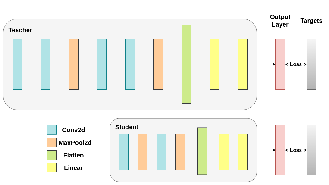
先用交叉熵训练两个网络。学生的结果作为后续比较的基线：

def train(model, train_loader, epochs, learning_rate, device):
    criterion = nn.CrossEntropyLoss()
    optimizer = optim.Adam(model.parameters(), lr=learning_rate)

    model.train()

    for epoch in range(epochs):
        running_loss = 0.0
        for inputs, labels in train_loader:
            # inputs: A collection of batch_size images
            # labels: A vector of dimensionality batch_size with integers denoting class of each image
            inputs, labels = inputs.to(device), labels.to(device)

            optimizer.zero_grad()
            outputs = model(inputs)

            # outputs: Output of the network for the collection of images. A tensor of dimensionality batch_size x num_classes
            # labels: The actual labels of the images. Vector of dimensionality batch_size
            loss = criterion(outputs, labels)
            loss.backward()
            optimizer.step()

            running_loss += loss.item()

        print(f"Epoch {epoch+1}/{epochs}, Loss: {running_loss / len(train_loader)}")

def test(model, test_loader, device):
    model.to(device)
    model.eval()

    correct = 0
    total = 0

    with torch.no_grad():
        for inputs, labels in test_loader:
            inputs, labels = inputs.to(device), labels.to(device)

            outputs = model(inputs)
            _, predicted = torch.max(outputs.data, 1)

            total += labels.size(0)
            correct += (predicted == labels).sum().item()

    accuracy = 100 * correct / total
    print(f"Test Accuracy: {accuracy:.2f}%")
    return accuracy

交叉熵实验

为便于复现，设置 PyTorch 的随机种子。不同方法之间要公平比较，应让对应学生模型具有相同的初始权重。先使用交叉熵训练教师网络：

torch.manual_seed(42)
nn_deep = DeepNN(num_classes=10).to(device)
train(nn_deep, train_loader, epochs=10, learning_rate=0.001, device=device)
test_accuracy_deep = test(nn_deep, test_loader, device)

# Instantiate the lightweight network:
torch.manual_seed(42)
nn_light = LightNN(num_classes=10).to(device)

Epoch 1/10, Loss: 1.3382342433380654
Epoch 2/10, Loss: 0.8701328546799663
Epoch 3/10, Loss: 0.6824112486503923
Epoch 4/10, Loss: 0.5369700851190425
Epoch 5/10, Loss: 0.41664083873676827
Epoch 6/10, Loss: 0.3101733888277922
Epoch 7/10, Loss: 0.22270960162591447
Epoch 8/10, Loss: 0.1736413350000101
Epoch 9/10, Loss: 0.13697378467911345
Epoch 10/10, Loss: 0.11983640344761064
Test Accuracy: 75.08%

再创建一个轻量模型，用来比较训练方法。反向传播对权重初始化敏感，因此要让这两个学生模型以相同的初始化开始。

torch.manual_seed(42)
new_nn_light = LightNN(num_classes=10).to(device)

原文通过检查第一层权重的范数，快速确认新实例的初始化。需要区分：相同随机种子与相同构造流程用于复现初始化；仅第一层范数相等，本身不能严格证明整个网络的全部权重相同。

# Print the norm of the first layer of the initial lightweight model
print("Norm of 1st layer of nn_light:", torch.norm(nn_light.features[0].weight).item())
# Print the norm of the first layer of the new lightweight model
print("Norm of 1st layer of new_nn_light:", torch.norm(new_nn_light.features[0].weight).item())

Norm of 1st layer of nn_light: 2.327361822128296
Norm of 1st layer of new_nn_light: 2.327361822128296

打印两个模型的总参数数量：

total_params_deep = "{:,}".format(sum(p.numel() for p in nn_deep.parameters()))
print(f"DeepNN parameters: {total_params_deep}")
total_params_light = "{:,}".format(sum(p.numel() for p in nn_light.parameters()))
print(f"LightNN parameters: {total_params_light}")

DeepNN parameters: 1,186,986
LightNN parameters: 267,738

使用交叉熵训练并测试轻量网络：

train(nn_light, train_loader, epochs=10, learning_rate=0.001, device=device)
test_accuracy_light_ce = test(nn_light, test_loader, device)

Epoch 1/10, Loss: 1.4707639043593346
Epoch 2/10, Loss: 1.1576078964011443
Epoch 3/10, Loss: 1.0184178518517244
Epoch 4/10, Loss: 0.9116543808861461
Epoch 5/10, Loss: 0.8344270890326146
Epoch 6/10, Loss: 0.7696182061644161
Epoch 7/10, Loss: 0.7024521170674688
Epoch 8/10, Loss: 0.647325016729667
Epoch 9/10, Loss: 0.5949938573953136
Epoch 10/10, Loss: 0.5434329890838975
Test Accuracy: 70.54%

现在可以根据原文的测试准确率，比较深层教师网络与轻量学生网络。此时学生尚未接受教师指导，结果来自它独立训练的表现。可以用以下代码展示这些指标：

print(f"Teacher accuracy: {test_accuracy_deep:.2f}%")
print(f"Student accuracy: {test_accuracy_light_ce:.2f}%")

Teacher accuracy: 75.08%
Student accuracy: 70.54%

知识蒸馏实验

接下来利用教师改善学生的测试准确率。两者都输出针对相同类别的概率分布，输出神经元数量也相同。知识蒸馏在常规交叉熵之外，加入一个根据教师 softmax 输出计算的损失。

其假设是：训练充分的教师，其输出激活包含学生可以学习的额外信息。原始研究指出，软目标中较小概率之间的比例也有价值，能帮助模型形成数据之间的相似性结构，让相似对象在表示空间中更接近。例如，在 CIFAR-10 中，看到了轮子的卡车可能被误认为汽车或飞机，但较不可能被误认为狗。所以有价值的信息不只是教师预测概率最大的类别，也包括整个输出分布。

只使用真实标签的交叉熵，往往不能充分利用这些信息。非主预测类别的激活可能很小，使得相应梯度不足以明显改变权重，形成希望获得的表示空间结构。

为引入教师与学生之间的训练关系，新的辅助函数增加以下参数：

• T：温度，控制输出分布的平滑程度。T 越大，分布越平滑，较小概率得到的相对提升越大。

• soft_target_loss_weight：给新增的软目标损失分配的权重。

• ce_loss_weight：交叉熵损失的权重。调整两项权重，会改变模型对两个训练目标的侧重。

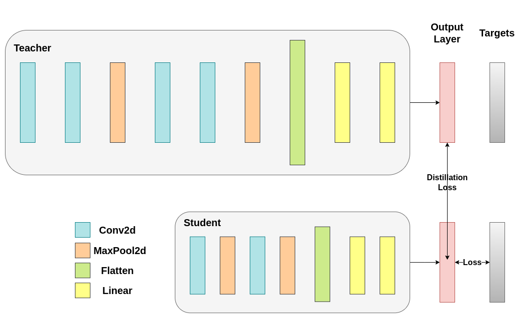
蒸馏损失根据教师和学生的 logits 计算，梯度只回传给学生：

def train_knowledge_distillation(teacher, student, train_loader, epochs, learning_rate, T, soft_target_loss_weight, ce_loss_weight, device):
    ce_loss = nn.CrossEntropyLoss()
    optimizer = optim.Adam(student.parameters(), lr=learning_rate)

    teacher.eval()  # Teacher set to evaluation mode
    student.train() # Student to train mode

    for epoch in range(epochs):
        running_loss = 0.0
        for inputs, labels in train_loader:
            inputs, labels = inputs.to(device), labels.to(device)

            optimizer.zero_grad()

            # Forward pass with the teacher model - do not save gradients here as we do not change the teacher's weights
            with torch.no_grad():
                teacher_logits = teacher(inputs)

            # Forward pass with the student model
            student_logits = student(inputs)

            #Soften the student logits by applying softmax first and log() second
            soft_targets = nn.functional.softmax(teacher_logits / T, dim=-1)
            soft_prob = nn.functional.log_softmax(student_logits / T, dim=-1)

            # Calculate the soft targets loss. Scaled by T**2 as suggested by the authors of the paper "Distilling the knowledge in a neural network"
            soft_targets_loss = torch.sum(soft_targets * (soft_targets.log() - soft_prob)) / soft_prob.size()[0] * (T**2)

            # Calculate the true label loss
            label_loss = ce_loss(student_logits, labels)

            # Weighted sum of the two losses
            loss = soft_target_loss_weight * soft_targets_loss + ce_loss_weight * label_loss

            loss.backward()
            optimizer.step()

            running_loss += loss.item()

        print(f"Epoch {epoch+1}/{epochs}, Loss: {running_loss / len(train_loader)}")

# Apply ``train_knowledge_distillation`` with a temperature of 2. Arbitrarily set the weights to 0.75 for CE and 0.25 for distillation loss.
train_knowledge_distillation(teacher=nn_deep, student=new_nn_light, train_loader=train_loader, epochs=10, learning_rate=0.001, T=2, soft_target_loss_weight=0.25, ce_loss_weight=0.75, device=device)
test_accuracy_light_ce_and_kd = test(new_nn_light, test_loader, device)

# Compare the student test accuracy with and without the teacher, after distillation
print(f"Teacher accuracy: {test_accuracy_deep:.2f}%")
print(f"Student accuracy without teacher: {test_accuracy_light_ce:.2f}%")
print(f"Student accuracy with CE + KD: {test_accuracy_light_ce_and_kd:.2f}%")

Epoch 1/10, Loss: 2.406461823626857
Epoch 2/10, Loss: 1.8879692225200135
Epoch 3/10, Loss: 1.665034802978301
Epoch 4/10, Loss: 1.5042838031983436
Epoch 5/10, Loss: 1.3802779210193077
Epoch 6/10, Loss: 1.2641536535509408
Epoch 7/10, Loss: 1.1679201334943552
Epoch 8/10, Loss: 1.0830097512515915
Epoch 9/10, Loss: 1.007507309736803
Epoch 10/10, Loss: 0.9328448636757444
Test Accuracy: 70.73%
Teacher accuracy: 75.08%
Student accuracy without teacher: 70.54%
Student accuracy with CE + KD: 70.73%

最小化余弦损失的实验

可以调整温度参数与损失系数，观察 softmax 分布平滑程度和训练目标权重的影响。神经网络中也可以在主要目标之外增加损失，尝试改善泛化能力。

下面把关注点从输出层移到隐藏状态。通过加入一个直接的损失，让卷积特征展平后、即将送入分类器的向量随着损失减小而变得更相似。教师不更新权重，优化只依赖学生的权重。

这种方法假设教师的内部表示更好，学生单靠自身训练不容易达到，所以推动学生模仿教师。但能否因此受益并不确定：教师表示如果有利于分类，模仿它可能有帮助；另一方面，两种网络架构和学习能力不同，强行匹配也可能有害。学生和教师的向量并没有逐分量对应的必然理由。例如，学生学到教师表示的一种排列，也可能同样有效。

仍然可以通过一个实验观察其影响。下面使用 CosineEmbeddingLoss，公式如下：

图：CosineEmbeddingLoss 的公式。

首先要解决维度问题。输出层蒸馏时，两个网络的输出神经元数量都等于类别数；但卷积层后的隐藏表示不是这样。最后一个卷积层的输出展平后，教师向量比学生更长。损失函数要求两个输入向量维度相同，因此在教师的卷积特征之后加入平均池化，降低维度，使它与学生一致。

为此修改或重新定义模型类：forward 不只返回 logits，还返回卷积特征展平后的隐藏表示。修改后的教师包含上述平均池化操作。

class ModifiedDeepNNCosine(nn.Module):
    def __init__(self, num_classes=10):
        super(ModifiedDeepNNCosine, self).__init__()
        self.features = nn.Sequential(
            nn.Conv2d(3, 128, kernel_size=3, padding=1),
            nn.ReLU(),
            nn.Conv2d(128, 64, kernel_size=3, padding=1),
            nn.ReLU(),
            nn.MaxPool2d(kernel_size=2, stride=2),
            nn.Conv2d(64, 64, kernel_size=3, padding=1),
            nn.ReLU(),
            nn.Conv2d(64, 32, kernel_size=3, padding=1),
            nn.ReLU(),
            nn.MaxPool2d(kernel_size=2, stride=2),
        )
        self.classifier = nn.Sequential(
            nn.Linear(2048, 512),
            nn.ReLU(),
            nn.Dropout(0.1),
            nn.Linear(512, num_classes)
        )

    def forward(self, x):
        x = self.features(x)
        flattened_conv_output = torch.flatten(x, 1)
        x = self.classifier(flattened_conv_output)
        flattened_conv_output_after_pooling = torch.nn.functional.avg_pool1d(flattened_conv_output, 2)
        return x, flattened_conv_output_after_pooling

# Create a similar student class where we return a tuple. We do not apply pooling after flattening.
class ModifiedLightNNCosine(nn.Module):
    def __init__(self, num_classes=10):
        super(ModifiedLightNNCosine, self).__init__()
        self.features = nn.Sequential(
            nn.Conv2d(3, 16, kernel_size=3, padding=1),
            nn.ReLU(),
            nn.MaxPool2d(kernel_size=2, stride=2),
            nn.Conv2d(16, 16, kernel_size=3, padding=1),
            nn.ReLU(),
            nn.MaxPool2d(kernel_size=2, stride=2),
        )
        self.classifier = nn.Sequential(
            nn.Linear(1024, 256),
            nn.ReLU(),
            nn.Dropout(0.1),
            nn.Linear(256, num_classes)
        )

    def forward(self, x):
        x = self.features(x)
        flattened_conv_output = torch.flatten(x, 1)
        x = self.classifier(flattened_conv_output)
        return x, flattened_conv_output

# We do not have to train the modified deep network from scratch of course, we just load its weights from the trained instance
modified_nn_deep = ModifiedDeepNNCosine(num_classes=10).to(device)
modified_nn_deep.load_state_dict(nn_deep.state_dict())

# Once again ensure the norm of the first layer is the same for both networks
print("Norm of 1st layer for deep_nn:", torch.norm(nn_deep.features[0].weight).item())
print("Norm of 1st layer for modified_deep_nn:", torch.norm(modified_nn_deep.features[0].weight).item())

# Initialize a modified lightweight network with the same seed as our other lightweight instances. This will be trained from scratch to examine the effectiveness of cosine loss minimization.
torch.manual_seed(42)
modified_nn_light = ModifiedLightNNCosine(num_classes=10).to(device)
print("Norm of 1st layer:", torch.norm(modified_nn_light.features[0].weight).item())

Norm of 1st layer for deep_nn: 7.520284175872803
Norm of 1st layer for modified_deep_nn: 7.520284175872803
Norm of 1st layer: 2.327361822128296

由于模型现在返回 (logits, hidden_representation)，训练循环也需要调整。先用一个样本输入打印两个返回张量的形状：

# Create a sample input tensor
sample_input = torch.randn(128, 3, 32, 32).to(device) # Batch size: 128, Filters: 3, Image size: 32x32

# Pass the input through the student
logits, hidden_representation = modified_nn_light(sample_input)

# Print the shapes of the tensors
print("Student logits shape:", logits.shape) # batch_size x total_classes
print("Student hidden representation shape:", hidden_representation.shape) # batch_size x hidden_representation_size

# Pass the input through the teacher
logits, hidden_representation = modified_nn_deep(sample_input)

# Print the shapes of the tensors
print("Teacher logits shape:", logits.shape) # batch_size x total_classes
print("Teacher hidden representation shape:", hidden_representation.shape) # batch_size x hidden_representation_size

Student logits shape: torch.Size([128, 10])
Student hidden representation shape: torch.Size([128, 1024])
Teacher logits shape: torch.Size([128, 10])
Teacher hidden representation shape: torch.Size([128, 1024])

这里的 hidden_representation_size 为 1024，对应学生最后一个卷积层展平后的特征，也是分类器的输入。教师原本为 2048，通过 avg_pool1d 降到 1024。

额外的隐藏表示损失只影响学生从输入到该表示之间的权重，不直接更新后面的分类器；分类器仍由分类交叉熵更新。修改后的训练循环如下：

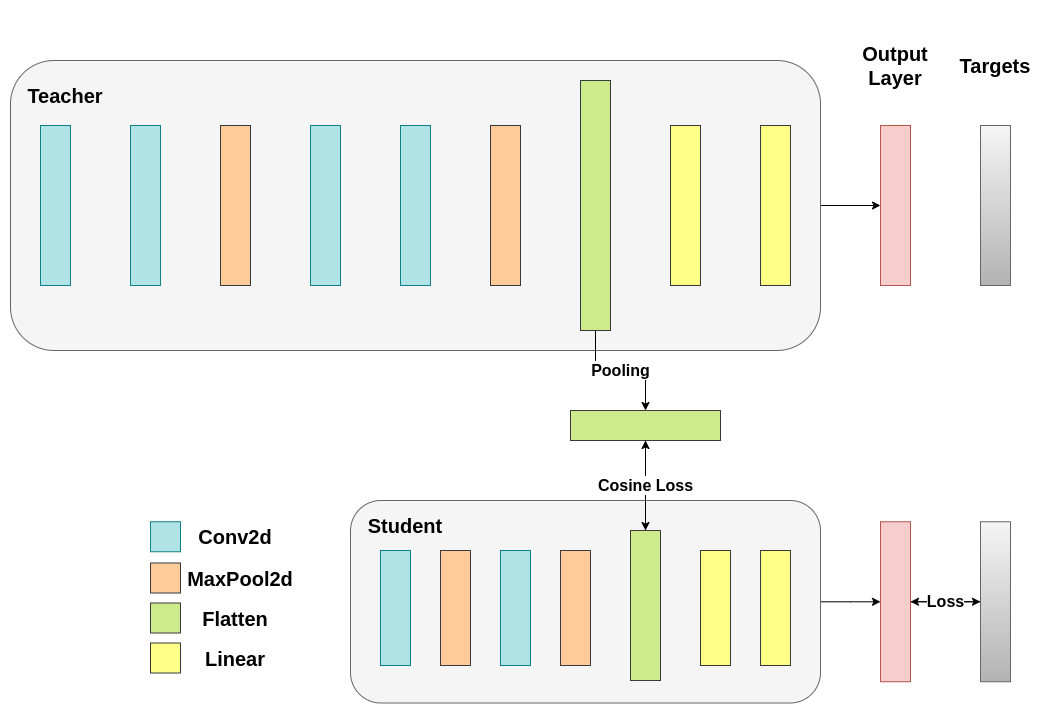
最小化余弦损失时，通过只向学生回传梯度，增大两个表示之间的余弦相似度：

def train_cosine_loss(teacher, student, train_loader, epochs, learning_rate, hidden_rep_loss_weight, ce_loss_weight, device):
    ce_loss = nn.CrossEntropyLoss()
    cosine_loss = nn.CosineEmbeddingLoss()
    optimizer = optim.Adam(student.parameters(), lr=learning_rate)

    teacher.to(device)
    student.to(device)
    teacher.eval()  # Teacher set to evaluation mode
    student.train() # Student to train mode

    for epoch in range(epochs):
        running_loss = 0.0
        for inputs, labels in train_loader:
            inputs, labels = inputs.to(device), labels.to(device)

            optimizer.zero_grad()

            # Forward pass with the teacher model and keep only the hidden representation
            with torch.no_grad():
                _, teacher_hidden_representation = teacher(inputs)

            # Forward pass with the student model
            student_logits, student_hidden_representation = student(inputs)

            # Calculate the cosine loss. Target is a vector of ones. From the loss formula above we can see that is the case where loss minimization leads to cosine similarity increase.
            hidden_rep_loss = cosine_loss(student_hidden_representation, teacher_hidden_representation, target=torch.ones(inputs.size(0)).to(device))

            # Calculate the true label loss
            label_loss = ce_loss(student_logits, labels)

            # Weighted sum of the two losses
            loss = hidden_rep_loss_weight * hidden_rep_loss + ce_loss_weight * label_loss

            loss.backward()
            optimizer.step()

            running_loss += loss.item()

        print(f"Epoch {epoch+1}/{epochs}, Loss: {running_loss / len(train_loader)}")

测试函数也需要相应调整，忽略模型返回的隐藏表示，只使用分类 logits：

def test_multiple_outputs(model, test_loader, device):
    model.to(device)
    model.eval()

    correct = 0
    total = 0

    with torch.no_grad():
        for inputs, labels in test_loader:
            inputs, labels = inputs.to(device), labels.to(device)

            outputs, _ = model(inputs) # Disregard the second tensor of the tuple
            _, predicted = torch.max(outputs.data, 1)

            total += labels.size(0)
            correct += (predicted == labels).sum().item()

    accuracy = 100 * correct / total
    print(f"Test Accuracy: {accuracy:.2f}%")
    return accuracy

同一个函数也可以同时加入输出知识蒸馏和隐藏表示余弦损失。在教师与学生训练中，组合多种方法很常见。这里先运行一个简单的训练与测试过程：

# Train and test the lightweight network with cross entropy loss
train_cosine_loss(teacher=modified_nn_deep, student=modified_nn_light, train_loader=train_loader, epochs=10, learning_rate=0.001, hidden_rep_loss_weight=0.25, ce_loss_weight=0.75, device=device)
test_accuracy_light_ce_and_cosine_loss = test_multiple_outputs(modified_nn_light, test_loader, device)

Epoch 1/10, Loss: 1.3062417119970102
Epoch 2/10, Loss: 1.0699138793798968
Epoch 3/10, Loss: 0.9699441549723106
Epoch 4/10, Loss: 0.8946081829802764
Epoch 5/10, Loss: 0.8405215176170134
Epoch 6/10, Loss: 0.7965446832539785
Epoch 7/10, Loss: 0.755501888597103
Epoch 8/10, Loss: 0.7213265583338335
Epoch 9/10, Loss: 0.6832332179674407
Epoch 10/10, Loss: 0.6572130263004157
Test Accuracy: 70.14%

中间回归器实验

这种直接最小化并不保证得到更好的结果。向量维度是原因之一：高维向量中，余弦相似度通常比欧氏距离更合适，但这里每个向量有 1024 个分量，从中提取有意义的相似性仍很困难。

此外，前面已经说明，没有理论依据要求学生与教师的隐藏向量逐分量一一匹配。最后一个例子加入额外的可训练回归器：先提取教师某个卷积层的特征图，再提取学生的特征图，让二者通过回归器对齐。

回归器为匹配过程提供可学习的调整空间，希望优于直接施加余弦损失。它首先使两个特征图维度相同，以便定义教师与学生之间的损失。这个损失构成一条教学路径，通过反向传播改变学生的权重。原始网络分类器之前的卷积特征具有以下形状：

# Pass the sample input only from the convolutional feature extractor
convolutional_fe_output_student = nn_light.features(sample_input)
convolutional_fe_output_teacher = nn_deep.features(sample_input)

# Print their shapes
print("Student's feature extractor output shape: ", convolutional_fe_output_student.shape)
print("Teacher's feature extractor output shape: ", convolutional_fe_output_teacher.shape)

Student's feature extractor output shape:  torch.Size([128, 16, 8, 8])
Teacher's feature extractor output shape:  torch.Size([128, 32, 8, 8])

教师有 32 个滤波器，学生有 16 个。加入可训练层，把学生特征图转换成教师特征图的形状。具体而言，修改轻量模型，让它返回经过中间回归器的隐藏特征；修改教师，让它返回最后卷积层的输出，不做额外池化或展平。

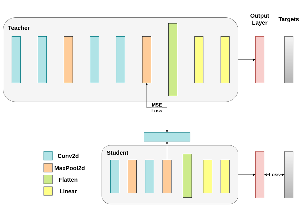
可训练层匹配了中间张量的形状，因而可以在两个特征图上正确计算均方误差（MSE）：

class ModifiedDeepNNRegressor(nn.Module):
    def __init__(self, num_classes=10):
        super(ModifiedDeepNNRegressor, self).__init__()
        self.features = nn.Sequential(
            nn.Conv2d(3, 128, kernel_size=3, padding=1),
            nn.ReLU(),
            nn.Conv2d(128, 64, kernel_size=3, padding=1),
            nn.ReLU(),
            nn.MaxPool2d(kernel_size=2, stride=2),
            nn.Conv2d(64, 64, kernel_size=3, padding=1),
            nn.ReLU(),
            nn.Conv2d(64, 32, kernel_size=3, padding=1),
            nn.ReLU(),
            nn.MaxPool2d(kernel_size=2, stride=2),
        )
        self.classifier = nn.Sequential(
            nn.Linear(2048, 512),
            nn.ReLU(),
            nn.Dropout(0.1),
            nn.Linear(512, num_classes)
        )

    def forward(self, x):
        x = self.features(x)
        conv_feature_map = x
        x = torch.flatten(x, 1)
        x = self.classifier(x)
        return x, conv_feature_map

class ModifiedLightNNRegressor(nn.Module):
    def __init__(self, num_classes=10):
        super(ModifiedLightNNRegressor, self).__init__()
        self.features = nn.Sequential(
            nn.Conv2d(3, 16, kernel_size=3, padding=1),
            nn.ReLU(),
            nn.MaxPool2d(kernel_size=2, stride=2),
            nn.Conv2d(16, 16, kernel_size=3, padding=1),
            nn.ReLU(),
            nn.MaxPool2d(kernel_size=2, stride=2),
        )
        # Include an extra regressor (in our case linear)
        self.regressor = nn.Sequential(
            nn.Conv2d(16, 32, kernel_size=3, padding=1)
        )
        self.classifier = nn.Sequential(
            nn.Linear(1024, 256),
            nn.ReLU(),
            nn.Dropout(0.1),
            nn.Linear(256, num_classes)
        )

    def forward(self, x):
        x = self.features(x)
        regressor_output = self.regressor(x)
        x = torch.flatten(x, 1)
        x = self.classifier(x)
        return x, regressor_output

再次修改训练循环：提取学生回归器的输出，以及教师特征图；对形状完全相同的张量计算 MSE，并据此反向传播梯度，同时保留分类任务的常规交叉熵损失。

def train_mse_loss(teacher, student, train_loader, epochs, learning_rate, feature_map_weight, ce_loss_weight, device):
    ce_loss = nn.CrossEntropyLoss()
    mse_loss = nn.MSELoss()
    optimizer = optim.Adam(student.parameters(), lr=learning_rate)

    teacher.to(device)
    student.to(device)
    teacher.eval()  # Teacher set to evaluation mode
    student.train() # Student to train mode

    for epoch in range(epochs):
        running_loss = 0.0
        for inputs, labels in train_loader:
            inputs, labels = inputs.to(device), labels.to(device)

            optimizer.zero_grad()

            # Again ignore teacher logits
            with torch.no_grad():
                _, teacher_feature_map = teacher(inputs)

            # Forward pass with the student model
            student_logits, regressor_feature_map = student(inputs)

            # Calculate the loss
            hidden_rep_loss = mse_loss(regressor_feature_map, teacher_feature_map)

            # Calculate the true label loss
            label_loss = ce_loss(student_logits, labels)

            # Weighted sum of the two losses
            loss = feature_map_weight * hidden_rep_loss + ce_loss_weight * label_loss

            loss.backward()
            optimizer.step()

            running_loss += loss.item()

        print(f"Epoch {epoch+1}/{epochs}, Loss: {running_loss / len(train_loader)}")

# Notice how our test function remains the same here with the one we used in our previous case. We only care about the actual outputs because we measure accuracy.

# Initialize a ModifiedLightNNRegressor
torch.manual_seed(42)
modified_nn_light_reg = ModifiedLightNNRegressor(num_classes=10).to(device)

# We do not have to train the modified deep network from scratch of course, we just load its weights from the trained instance
modified_nn_deep_reg = ModifiedDeepNNRegressor(num_classes=10).to(device)
modified_nn_deep_reg.load_state_dict(nn_deep.state_dict())

# Train and test once again
train_mse_loss(teacher=modified_nn_deep_reg, student=modified_nn_light_reg, train_loader=train_loader, epochs=10, learning_rate=0.001, feature_map_weight=0.25, ce_loss_weight=0.75, device=device)
test_accuracy_light_ce_and_mse_loss = test_multiple_outputs(modified_nn_light_reg, test_loader, device)

Epoch 1/10, Loss: 1.7166156210862766
Epoch 2/10, Loss: 1.337869451478924
Epoch 3/10, Loss: 1.195537436953591
Epoch 4/10, Loss: 1.100342325237401
Epoch 5/10, Loss: 1.0221911214501656
Epoch 6/10, Loss: 0.9601379102453247
Epoch 7/10, Loss: 0.9062253306893742
Epoch 8/10, Loss: 0.8578306328305199
Epoch 9/10, Loss: 0.8180762854073663
Epoch 10/10, Loss: 0.7783686616231719
Test Accuracy: 70.89%

由于加入了教师与学生之间的可训练层，学生有更大的学习调整空间，而不是被迫直接复制教师表示，所以原文预期这一方法优于直接使用 CosineLoss。这仍是实验预期，不能保证普遍改善。加入辅助网络也是基于提示的蒸馏（hint-based distillation）的核心思路。

print(f"Teacher accuracy: {test_accuracy_deep:.2f}%")
print(f"Student accuracy without teacher: {test_accuracy_light_ce:.2f}%")
print(f"Student accuracy with CE + KD: {test_accuracy_light_ce_and_kd:.2f}%")
print(f"Student accuracy with CE + CosineLoss: {test_accuracy_light_ce_and_cosine_loss:.2f}%")
print(f"Student accuracy with CE + RegressorMSE: {test_accuracy_light_ce_and_mse_loss:.2f}%")

Teacher accuracy: 75.08%
Student accuracy without teacher: 70.54%
Student accuracy with CE + KD: 70.73%
Student accuracy with CE + CosineLoss: 70.14%
Student accuracy with CE + RegressorMSE: 70.89%

结论

这些训练目标可以把教师的信息传递给轻量学生，而部署时通常只需要学生的分类分支。需要明确，回归器示例增加了辅助参数，而且原样 forward 仍会计算该分支；只有部署时移除不需要的辅助分支，才能讨论分类网络推理成本保持不变。训练阶段则需要额外计算教师前向过程和辅助损失。

模型部署后通常更关注推理开销。如果轻量模型仍不适合目标设备，还可以考虑训练后量化。额外损失也不局限于分类任务，可以尝试不同损失系数、温度或神经元数量。不过，修改神经元或滤波器数量时，容易造成张量形状不匹配，应相应检查对齐方式。

原文各次准确率来自它展示的实验，不能作为本机结果或普遍性能保证。多次比较方法时，应保留独立的最终测试集，以减少反复试验造成的选择偏差。

进一步阅读：

• Hinton、Vinyals、Dean：Distilling the Knowledge in a Neural Network，2015。

• Romero 等：FitNets: Hints for Thin Deep Nets，2015。

原文展示的脚本总运行时间为 4 分 35.285 秒。这是原文环境中的记录，不代表其他设备或本机的耗时。

下载原文 Jupyter notebook：knowledge_distillation_tutorial.ipynb。

下载原文 Python 源码：knowledge_distillation_tutorial.py。

下载原文 ZIP：knowledge_distillation_tutorial.zip。

来源与许可

原文：Knowledge Distillation Tutorial。作者或贡献者：Alexandros Chariton / PyTorch contributors。本中文版本为翻译；代码、注释和原文示例输出保留原样，必要的技术澄清已在相应段落说明。适用许可：BSD-3-Clause。

许可原文

BSD 3-Clause License

Copyright (c) 2017-2022, Pytorch contributors All rights reserved.

Redistribution and use in source and binary forms, with or without modification, are permitted provided that the following conditions are met:

• Redistributions of source code must retain the above copyright notice, this list of conditions and the following disclaimer.

• Redistributions in binary form must reproduce the above copyright notice, this list of conditions and the following disclaimer in the documentation and/or other materials provided with the distribution.

• Neither the name of the copyright holder nor the names of its contributors may be used to endorse or promote products derived from this software without specific prior written permission.

THIS SOFTWARE IS PROVIDED BY THE COPYRIGHT HOLDERS AND CONTRIBUTORS “AS IS” AND ANY EXPRESS OR IMPLIED WARRANTIES, INCLUDING, BUT NOT LIMITED TO, THE IMPLIED WARRANTIES OF MERCHANTABILITY AND FITNESS FOR A PARTICULAR PURPOSE ARE DISCLAIMED. IN NO EVENT SHALL THE COPYRIGHT HOLDER OR CONTRIBUTORS BE LIABLE FOR ANY DIRECT, INDIRECT, INCIDENTAL, SPECIAL, EXEMPLARY, OR CONSEQUENTIAL DAMAGES (INCLUDING, BUT NOT LIMITED TO, PROCUREMENT OF SUBSTITUTE GOODS OR SERVICES; LOSS OF USE, DATA, OR PROFITS; OR BUSINESS INTERRUPTION) HOWEVER CAUSED AND ON ANY THEORY OF LIABILITY, WHETHER IN CONTRACT, STRICT LIABILITY, OR TORT (INCLUDING NEGLIGENCE OR OTHERWISE) ARISING IN ANY WAY OUT OF THE USE OF THIS SOFTWARE, EVEN IF ADVISED OF THE POSSIBILITY OF SUCH DAMAGE.