用 SciPy 构造并核查二维点集的几何分区

原文：Spatial Data Structures and Algorithms (scipy.spatial)，SciPy 1.18.0 官方手册，作者为 SciPy 文档贡献者。本文完整翻译三角剖分、凸包、Voronoi 分区及生成图案例子，代码与交互输出保留原文形式。

scipy.spatial 借助 Qhull，可以计算点集的三角剖分、Voronoi 图和凸包。它还提供用于最近邻点查询的 KDTree 实现，以及在不同度量下计算距离的工具。

阅读前提：示例使用 NumPy、SciPy 和 Matplotlib。带 >>>、... 的代码块是交互式 Python 会话：提示符后为输入，未带提示符的数组等内容是原站示例输出。复制到脚本时需区分输入与输出，并移除提示符；本文未执行这些代码。

Delaunay 三角剖分

Delaunay 三角剖分将一组点划分为互不重叠的三角形，并满足：任何一个三角形的外接圆内部，都不包含点集中的其他点。在实践中，这类剖分往往避免出现很小的内角。

用 scipy.spatial 计算四点的 Delaunay 三角剖分：

>>> from scipy.spatial import Delaunay
>>> import numpy as np
>>> points = np.array([[0, 0], [0, 1.1], [1, 0], [1, 1]])
>>> tri = Delaunay(points)

可以这样绘制剖分结果：

>>> import matplotlib.pyplot as plt
>>> plt.triplot(points[:,0], points[:,1], tri.simplices)
>>> plt.plot(points[:,0], points[:,1], 'o')

再标注点编号与三角形编号，并设置坐标范围：

>>> for j, p in enumerate(points):
...     plt.text(p[0]-0.03, p[1]+0.03, j, ha='right') # label the points
>>> for j, s in enumerate(tri.simplices):
...     p = points[s].mean(axis=0)
...     plt.text(p[0], p[1], '#%d' % j, ha='center') # label triangles
>>> plt.xlim(-0.5, 1.5); plt.ylim(-0.5, 1.5)
>>> plt.show()

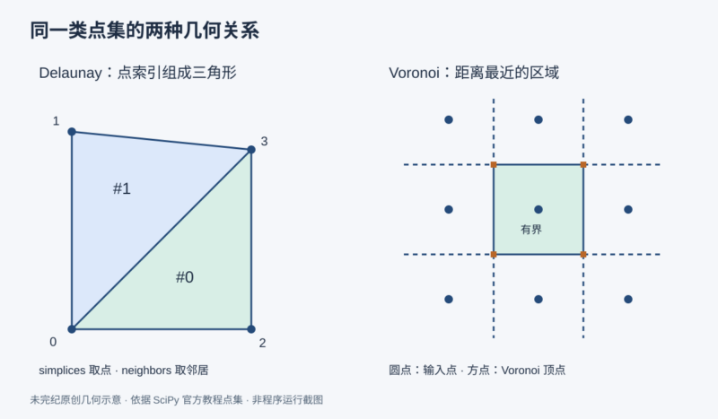
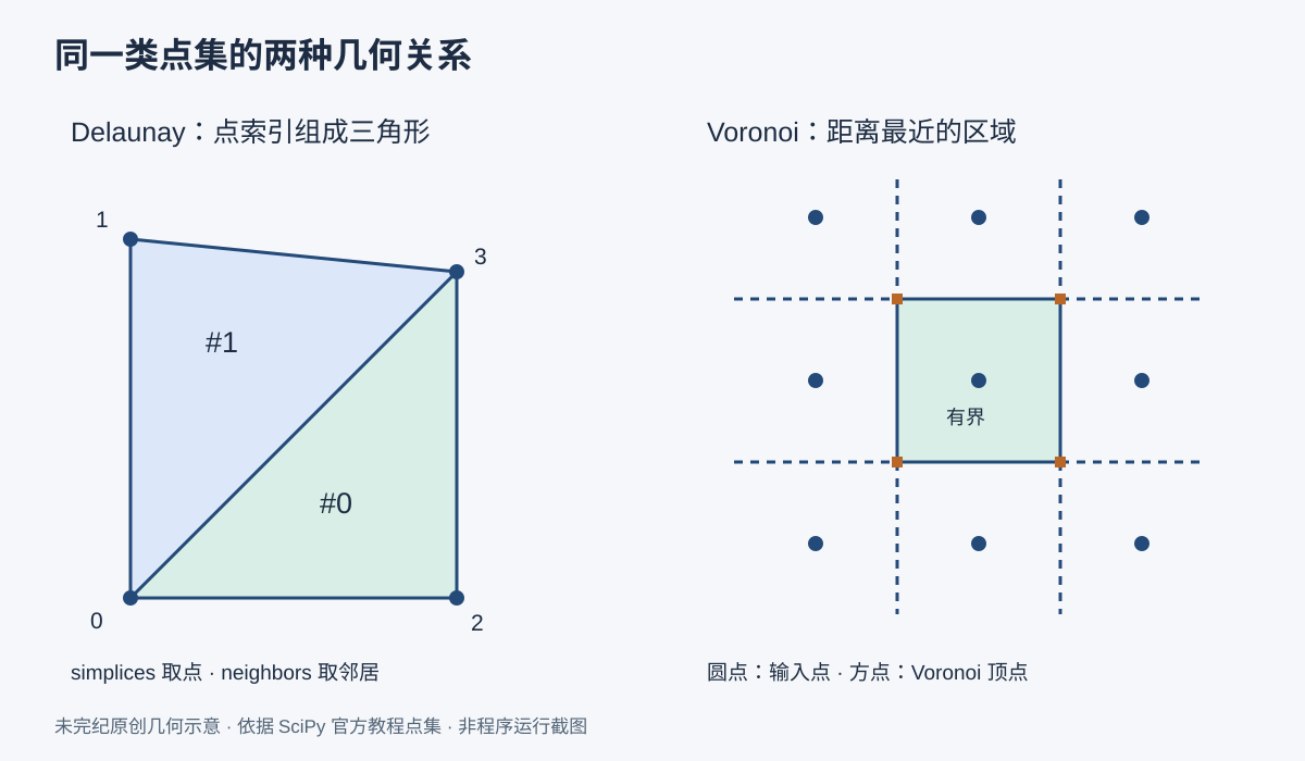
原图中，四个点大致构成一个四边形；点 0 和点 3 之间的对角线将其分成两个相邻三角形。上方三角形标为 #1，下方标为 #0。

剖分的结构编码在对象属性中。simplices 保存组成各三角形的点在 points 数组中的索引。例如：

>>> i = 1
>>> tri.simplices[i,:]
array([3, 1, 0], dtype=int32)
>>> points[tri.simplices[i,:]]
array([[ 1. ,  1. ],
       [ 0. ,  1.1],
       [ 0. ,  0. ]])

还可以查询相邻三角形：

>>> tri.neighbors[i]
array([-1,  0, -1], dtype=int32)

这个输出表示：该三角形有一个相邻三角形 #0，另外两条边没有相邻三角形，用 -1 表示。邻接数组中局部索引为 1（即第二个）的顶点所对的边，对应邻居 #0；这个顶点是：

>>> points[tri.simplices[i, 1]]
array([ 0. ,  1.1])

从原图也能看出这一关系。这里的局部顶点位置和 points 全局索引是两回事，核对时应先经由 tri.simplices 取回点。Qhull 也能对更高维的点集进行单纯形剖分，例如将三维点集分割为四面体。

共面点与退化情况

由于计算剖分时的数值精度问题，不一定所有输入点都会成为剖分的顶点。将上例换成含有重复点的点集：

>>> points = np.array([[0, 0], [0, 1], [1, 0], [1, 1], [1, 1]])
>>> tri = Delaunay(points)
>>> np.unique(tri.simplices.ravel())
array([0, 1, 2, 3], dtype=int32)

点 #4 与另一个点重复，因此没有作为顶点出现在剖分中。这件事会记录在 coplanar 中：

>>> tri.coplanar
array([[4, 0, 3]], dtype=int32)

其含义是：点 4 位于三角形 0、顶点 3 附近，但没有被纳入剖分。这类退化不只会由重复点引起；更复杂的几何关系也可能造成退化，即便点集看起来并没有明显问题。

Qhull 提供 QJ 选项，会随机扰动输入数据，直至退化情况得到处理：

>>> tri = Delaunay(points, qhull_options="QJ Pp")
>>> points[tri.simplices]
array([[[1, 0],
        [1, 1],
        [0, 0]],
       [[1, 1],
        [1, 1],
        [1, 0]],
       [[1, 1],
        [0, 1],
        [0, 0]],
       [[0, 1],
        [1, 1],
        [1, 1]]])

这里多出了两个三角形。不过，将索引映射回原始点坐标后，可以看到它们仍是退化的，面积为零。扰动使算法完成剖分，不等于原始点集中的每个三角形都获得了非零面积。

凸包

凸包是包含给定点集所有点的最小凸对象。通过 scipy.spatial 对 Qhull 的封装，可以这样计算：

>>> from scipy.spatial import ConvexHull
>>> rng = np.random.default_rng()
>>> points = rng.random((30, 2))   # 30 random points in 2-D
>>> hull = ConvexHull(points)

这里生成 30 个二维随机点。凸包以一组一维单纯形表示；在二维中，一维单纯形就是线段。它的存储方案与上面的 Delaunay 单纯形完全相同，仍然通过点索引表示。

下面把点集和凸包边界画出来：

>>> import matplotlib.pyplot as plt
>>> plt.plot(points[:,0], points[:,1], 'o')
>>> for simplex in hull.simplices:
...     plt.plot(points[simplex,0], points[simplex,1], 'k-')
>>> plt.show()

图中的黑色线段围住所有点。同样的效果也可以用 scipy.spatial.convex_hull_plot_2d 得到。原文随机数生成器未指定种子，重新运行时点的位置和凸包边界会改变。

Voronoi 图：按最近的输入点划分空间

Voronoi 图将空间分成给定点集的最近邻区域。scipy.spatial 提供两种处理思路。

先用 KDTree 回答最近邻查询

第一种方式使用 KDTree 回答“输入点中哪个点离查询位置最近”，由此定义区域：

>>> from scipy.spatial import KDTree
>>> points = np.array([[0, 0], [0, 1], [0, 2], [1, 0], [1, 1], [1, 2],
...                    [2, 0], [2, 1], [2, 2]])
>>> tree = KDTree(points)
>>> tree.query([0.1, 0.1])
(0.14142135623730953, 0)

因此位置 (0.1, 0.1) 属于区域 0；返回值第一项是距离，第二项是最近点的索引。可以把区域按颜色画出来：

>>> x = np.linspace(-0.5, 2.5, 31)
>>> y = np.linspace(-0.5, 2.5, 33)
>>> xx, yy = np.meshgrid(x, y)
>>> xy = np.c_[xx.ravel(), yy.ravel()]
>>> import matplotlib.pyplot as plt
>>> dx_half, dy_half = np.diff(x[:2])[0] / 2., np.diff(y[:2])[0] / 2.
>>> x_edges = np.concatenate((x - dx_half, [x[-1] + dx_half]))
>>> y_edges = np.concatenate((y - dy_half, [y[-1] + dy_half]))
>>> plt.pcolormesh(x_edges, y_edges, tree.query(xy)[1].reshape(33, 31), shading='flat')
>>> plt.plot(points[:,0], points[:,1], 'ko')
>>> plt.show()

这段代码在 x 方向取 31 个采样位置、y 方向取 33 个，拼成网格后批量查询最近点，再将返回的索引恢复为 33×31 的二维数组。x_edges 和 y_edges 从采样点向外扩展半格，给 pcolormesh 的平坦着色提供单元边界。

这样得到了最近邻区域的颜色图，但还没有得到作为几何对象的 Voronoi 图：图形本身的顶点、线段和无界边尚未显式给出。

用 Voronoi 对象取得顶点与区域

再一次使用 Qhull 的封装，可以得到线和点形式的表示：

>>> from scipy.spatial import Voronoi
>>> vor = Voronoi(points)
>>> vor.vertices
array([[0.5, 0.5],
       [0.5, 1.5],
       [1.5, 0.5],
       [1.5, 1.5]])

Voronoi 顶点构成各区域的多边形边界。在这个例子中，共有九个不同区域：

>>> vor.regions
[[], [-1, 0], [-1, 1], [1, -1, 0], [3, -1, 2], [-1, 3], [-1, 2], [0, 1, 3, 2], [2, -1, 0], [3, -1, 1]]

-1 再次表示无穷远处的顶点。这里只有 [0, 1, 3, 2] 对应的区域有界，其余区域向无穷延伸。与前面 Delaunay 剖分的精度问题类似，Voronoi 区域数量也可能少于输入点数量。

编辑补充：regions 示例开头的空列表不表示又多了一个有效输入点区域；不要直接把列表位置当成输入点索引。若要建立点到区域的对应，应查询对象的 point_region。这里不把示例的顶点或区域编号当成跨版本、跨数据的固定保证。

读取分隔区域的脊线

分隔区域的脊线（ridge，在二维中是线）也使用类似凸包边的单纯形集合来描述：

>>> vor.ridge_vertices
[[-1, 0], [-1, 0], [-1, 1], [-1, 1], [0, 1], [-1, 3], [-1, 2], [2, 3], [-1, 3], [-1, 2], [1, 3], [0, 2]]

这些数值是构成线段的 Voronoi 顶点索引。-1 仍表示无穷远，因此 12 条边中只有 4 条是有界线段，其余都延伸到无穷。

Voronoi 脊线垂直于相应两个输入点之间的连线。每条脊线对应哪两个输入点，也被记录下来：

>>> vor.ridge_points
array([[0, 3],
       [0, 1],
       [2, 5],
       [2, 1],
       [1, 4],
       [7, 8],
       [7, 6],
       [7, 4],
       [8, 5],
       [6, 3],
       [4, 5],
       [4, 3]], dtype=int32)

把这些信息结合起来，就足以构造整张图。

分别绘制有限边与无界边

先画原始点和 Voronoi 顶点，并确定坐标范围：

>>> plt.plot(points[:, 0], points[:, 1], 'o')
>>> plt.plot(vor.vertices[:, 0], vor.vertices[:, 1], '*')
>>> plt.xlim(-1, 3); plt.ylim(-1, 3)

绘制有界线段的方法与凸包类似，但现在要排除无穷端点：

>>> for simplex in vor.ridge_vertices:
...     simplex = np.asarray(simplex)
...     if np.all(simplex >= 0):
...         plt.plot(vor.vertices[simplex, 0], vor.vertices[simplex, 1], 'k-')

对于延伸到无穷的边，需要再做一些处理：

>>> center = points.mean(axis=0)
>>> for pointidx, simplex in zip(vor.ridge_points, vor.ridge_vertices):
...     simplex = np.asarray(simplex)
...     if np.any(simplex < 0):
...         i = simplex[simplex >= 0][0] # finite end Voronoi vertex
...         t = points[pointidx[1]] - points[pointidx[0]]  # tangent
...         t = t / np.linalg.norm(t)
...         n = np.array([-t[1], t[0]]) # normal
...         midpoint = points[pointidx].mean(axis=0)
...         far_point = vor.vertices[i] + np.sign(np.dot(midpoint - center, n)) * n * 100
...         plt.plot([vor.vertices[i,0], far_point[0]],
...                  [vor.vertices[i,1], far_point[1]], 'k--')
>>> plt.show()

代码先计算输入点集的中心。对带有负索引的脊线，取出有限端点；相应两个输入点的差向量给出切向方向 t，归一化后旋转得到法向 n。通过输入点中点相对中心的位置，选择朝外的法向符号，再从有限 Voronoi 顶点沿该方向延长 100 个单位，以虚线绘制。

这只是用于当前图形范围的绘图手法，数字 100 不是真正的“无穷大”，也没有把无界区域截成正式几何多边形。同样的图可以用 scipy.spatial.voronoi_plot_2d 绘制。

用 Voronoi 分区生成曼荼罗图案

Voronoi 图还可以用来创作有趣的生成艺术。尝试改变下面 mandala 函数的设置，构造自己的图案：

>>> import numpy as np
>>> from scipy import spatial
>>> import matplotlib.pyplot as plt

>>> def mandala(n_iter, n_points, radius):
...     """Creates a mandala figure using Voronoi tessellations.
...
...     Parameters
...     ----------
...     n_iter : int
...         Number of iterations, i.e. how many times the equidistant points will
...         be generated.
...     n_points : int
...         Number of points to draw per iteration.
...     radius : scalar
...         The radial expansion factor.
...
...     Returns
...     -------
...     fig : matplotlib.Figure instance
...
...     Notes
...     -----
...     This code is adapted from the work of Audrey Roy Greenfeld [1]_ and Carlos
...     Focil-Espinosa [2]_, who created beautiful mandalas with Python code.  That
...     code in turn was based on Antonio Sánchez Chinchón's R code [3]_.
...
...     References
...     ----------
...     .. [1] https://www.codemakesmehappy.com/2019/09/voronoi-mandalas.html
...
...     .. [2] https://github.com/CarlosFocil/mandalapy
...
...     .. [3] https://github.com/aschinchon/mandalas
...
...     """
...     fig = plt.figure(figsize=(10, 10))
...     ax = fig.add_subplot(111)
...     ax.set_axis_off()
...     ax.set_aspect('equal', adjustable='box')
...
...     angles = np.linspace(0, 2*np.pi * (1 - 1/n_points), num=n_points) + np.pi/2
...     # Starting from a single center point, add points iteratively
...     xy = np.array([[0, 0]])
...     for k in range(n_iter):
...         t1 = np.array([])
...         t2 = np.array([])
...         # Add `n_points` new points around each existing point in this iteration
...         for i in range(xy.shape[0]):
...             t1 = np.append(t1, xy[i, 0] + radius**k * np.cos(angles))
...             t2 = np.append(t2, xy[i, 1] + radius**k * np.sin(angles))
...
...         xy = np.column_stack((t1, t2))
...
...     # Create the Mandala figure via a Voronoi plot
...     spatial.voronoi_plot_2d(spatial.Voronoi(xy), ax=ax)
...
...     return fig

函数参数 n_iter 是迭代次数，也就是重复生成等距点的次数；n_points 是每次围绕一个已有点生成的点数；radius 是径向扩展因子。它返回一个 Matplotlib Figure。

函数从单个中心点开始，按角度均匀分布点。每一轮围绕上一轮的每个点添加新点，然后用新生成的坐标替换 xy；最后对点集计算 Voronoi 图。源码中的注释、文档字符串及引用均保留原文，以便追溯改编关系。

原文明确说明：这一代码改编自 Audrey Roy Greenfeld 的 Voronoi Mandalas 与 Carlos Focil-Espinosa 的 mandalapy，而两者又基于 Antonio Sánchez Chinchón 的 R 代码。这些归属不能从改编代码中删除。

原文使用以下参数生成示例：

>>> # Modify the following parameters in order to get different figures
>>> n_iter = 3
>>> n_points = 6
>>> radius = 4

>>> fig = mandala(n_iter, n_points, radius)
>>> plt.show()

通过调整迭代次数、点数和扩展因子，可得到不同的对称图案。图形由算法生成，本文未在本机重现原站的艺术图。

静态审查与复现注意事项

本次依据 SciPy 1.18.0 手册审查，原文没有为 NumPy 和 Matplotlib 锁定完整环境；不同 Qhull／SciPy 版本或输入顺序可能改变单纯形、区域与脊线编号。原站输出用于解释结构，不能用逐字匹配编号代替几何正确性检查。

输入均为内嵌数组或随机点，没有外部文件、网络请求、系统命令或凭据操作。真实数据仍需要核对维度、有限值、重复点、共线／共面情形和坐标尺度。无界边示例假设每条相应脊线具有可用的有限顶点，切向量长度非零；它针对本文二维点集，不能未经检查就套用到任意退化输入或高维数据。

曼荼罗函数每轮点数按 n_points 倍增长，最终规模约为 n_points ** n_iter。过大的参数会快速消耗内存与计算时间；n_points=0 还会使角度表达式除零。函数没有输入校验，实验时应从原文的小规模参数开始，并自行处理无效值。这些是静态审查发现的适用限制，并非本次运行测试结果。

中文翻译与原创几何示意：未完纪。SciPy 文档页署名 © The SciPy community；原文未给出个人作者或首次发表日期。随原示例保留以下项目许可声明。

代码许可证保留

项目 BSD 3-Clause 许可证：

Copyright (c) 2001-2002 Enthought, Inc. 2003, SciPy Developers.
All rights reserved.

Redistribution and use in source and binary forms, with or without
modification, are permitted provided that the following conditions
are met:

1. Redistributions of source code must retain the above copyright
   notice, this list of conditions and the following disclaimer.
2. Redistributions in binary form must reproduce the above
   copyright notice, this list of conditions and the following
   disclaimer in the documentation and/or other materials provided
   with the distribution.
3. Neither the name of the copyright holder nor the names of its
   contributors may be used to endorse or promote products derived
   from this software without specific prior written permission.

THIS SOFTWARE IS PROVIDED BY THE COPYRIGHT HOLDERS AND CONTRIBUTORS
"AS IS" AND ANY EXPRESS OR IMPLIED WARRANTIES, INCLUDING, BUT NOT
LIMITED TO, THE IMPLIED WARRANTIES OF MERCHANTABILITY AND FITNESS FOR
A PARTICULAR PURPOSE ARE DISCLAIMED. IN NO EVENT SHALL THE COPYRIGHT
OWNER OR CONTRIBUTORS BE LIABLE FOR ANY DIRECT, INDIRECT, INCIDENTAL,
SPECIAL, EXEMPLARY, OR CONSEQUENTIAL DAMAGES (INCLUDING, BUT NOT
LIMITED TO, PROCUREMENT OF SUBSTITUTE GOODS OR SERVICES; LOSS OF USE,
DATA, OR PROFITS; OR BUSINESS INTERRUPTION) HOWEVER CAUSED AND ON ANY
THEORY OF LIABILITY, WHETHER IN CONTRACT, STRICT LIABILITY, OR TORT
(INCLUDING NEGLIGENCE OR OTHERWISE) ARISING IN ANY WAY OUT OF THE USE
OF THIS SOFTWARE, EVEN IF ADVISED OF THE POSSIBILITY OF SUCH DAMAGE.