用 Julia 有限体积法模拟方形薄板的热扩散

原文：Diffusion Equation on a Square Plate，FiniteVolumeMethod.jl 官方文档。本文完整翻译方程、网格、边界条件、求解和绘图步骤，并保留原站代码及输出；编辑说明另行标注。

问题：一块上下初温不同的方形薄板

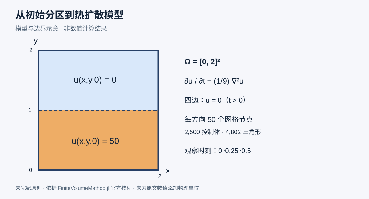
考虑正方形区域 Ω = [0, 2]² 上的扩散方程：

其中 x 表示位置向量 (x, y)，初始场按纵坐标分成两部分：

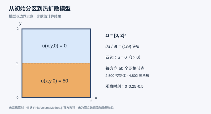
也就是说，扩散系数固定为 1/9，薄板边界在 t > 0 时保持零值，初始时下半部为 50、上半部为 0。原文未规定物理单位，不应为这些数值擅自添加摄氏度、米或秒等单位。

先定义网格

求解的第一步是创建网格。导入 FiniteVolumeMethod 和 DelaunayTriangulation，指定矩形的左右、上下界以及两个方向各 50 个节点，再将三角剖分包装为 FVMGeometry：

using FiniteVolumeMethod, DelaunayTriangulation
a, b, c, d = 0.0, 2.0, 0.0, 2.0
nx, ny = 50, 50
tri = triangulate_rectangle(a, b, c, d, nx, ny, single_boundary=true)
mesh = FVMGeometry(tri)

原站示例输出：

FVMGeometry with 2500 control volumes, 4802 triangles, and 7301 edges

这表示网格包含 2,500 个控制体、4,802 个三角形和 7,301 条边。下面使用 CairoMakie 显示该三角网格：

using CairoMakie
fig, ax, sc = triplot(tri)
fig

原文此处展示整个正方形被细密三角形覆盖的网格图。这里的 triplot(tri) 会根据实际三角剖分生成网格图；本文示意图用于解释几何条件，不替代它的运行结果。

定义齐次 Dirichlet 边界条件

边界上的解为零，因此使用齐次 Dirichlet 条件：

bc = (x, y, t, u, p) -> zero(u)
BCs = BoundaryConditions(mesh, bc, Dirichlet)

原站输出：

BoundaryConditions with 1 boundary condition with type Dirichlet

bc 的参数顺序为位置 x, y、时间 t、当前值 u 和参数 p；此处返回 zero(u)。single_boundary=true 将矩形边界作为一段边界处理，因此示例报告一个 Dirichlet 边界条件。

定义初始条件与扩散函数

接下来定义 PDE 本身。首先创建初值函数，再按三角剖分的点顺序形成初始值向量，最后定义扩散系数：

f = (x, y) -> y ≤ 1.0 ? 50.0 : 0.0
initial_condition = [f(x, y) for (x, y) in DelaunayTriangulation.each_point(tri)]
D = (x, y, t, u, p) -> 1 / 9

原站交互输出是 Julia 为最后创建的匿名函数显示的标识：

#7 (generic function with 1 method)

匿名函数编号与会话有关，不属于可依赖的计算结果。随后指定最终时间为 0.5，并构造问题：

final_time = 0.5
prob = FVMProblem(mesh, BCs; diffusion_function=D, initial_condition, final_time)

原站输出：

FVMProblem with 2500 nodes and time span (0.0, 0.5)

扩散函数会被转换为通量函数

需要注意，prob 内部使用的是通量函数，而不是直接使用扩散函数。可以查看：

prob.flux_function

原站输出：

#65 (generic function with 1 method)

提供 diffusion_function 后，通量为 q(x, t, α, β, γ) = (−α/9, −β/9)ᵀ。这里 (α, β, γ) 通过线性函数 u(x, y) = αx + βy + γ 定义对解的近似，因此梯度 ∇u = (α, β)ᵀ。负号表示通量沿场值下降的方向。

调用时间积分器求解

现在调用 solve。原文说明下述调用默认启用多线程；实际可使用的线程数仍取决于 Julia 的启动配置和运行环境。

using OrdinaryDiffEq
sol = solve(prob, Tsit5(), saveat=0.05)

这里显式选择 Tsit5()，并设置 saveat=0.05。若不确定选用哪个算法，原文建议改为 using DifferentialEquations，随后调用 solve(prob, saveat=0.05)，由工具自动选择算法。

下面是原站保留的输出，不是本次执行验证：

retcode: Success
Interpolation: 1st order linear
t: 11-element Vector{Float64}:
 0.0
 0.05
 0.1
 0.15
 0.2
 0.25
 0.3
 0.35
 0.4
 0.45
 0.5
u: 11-element Vector{Vector{Float64}}:
 [50.0, 50.0, 50.0, 50.0, 50.0, 50.0, 50.0, 50.0, 50.0, 50.0  …  0.0, 0.0, 0.0, 0.0, 0.0, 0.0, 0.0, 0.0, 0.0, 0.0]
 [0.0, 0.0, 0.0, 0.0, 0.0, 0.0, 0.0, 0.0, 0.0, 0.0  …  0.0, 0.0, 0.0, 0.0, 0.0, 0.0, 0.0, 0.0, 0.0, 0.0]
 [0.0, 0.0, 0.0, 0.0, 0.0, 0.0, 0.0, 0.0, 0.0, 0.0  …  0.0, 0.0, 0.0, 0.0, 0.0, 0.0, 0.0, 0.0, 0.0, 0.0]
 [0.0, 0.0, 0.0, 0.0, 0.0, 0.0, 0.0, 0.0, 0.0, 0.0  …  0.0, 0.0, 0.0, 0.0, 0.0, 0.0, 0.0, 0.0, 0.0, 0.0]
 [0.0, 0.0, 0.0, 0.0, 0.0, 0.0, 0.0, 0.0, 0.0, 0.0  …  0.0, 0.0, 0.0, 0.0, 0.0, 0.0, 0.0, 0.0, 0.0, 0.0]
 [0.0, 0.0, 0.0, 0.0, 0.0, 0.0, 0.0, 0.0, 0.0, 0.0  …  0.0, 0.0, 0.0, 0.0, 0.0, 0.0, 0.0, 0.0, 0.0, 0.0]
 [0.0, 0.0, 0.0, 0.0, 0.0, 0.0, 0.0, 0.0, 0.0, 0.0  …  0.0, 0.0, 0.0, 0.0, 0.0, 0.0, 0.0, 0.0, 0.0, 0.0]
 [0.0, 0.0, 0.0, 0.0, 0.0, 0.0, 0.0, 0.0, 0.0, 0.0  …  0.0, 0.0, 0.0, 0.0, 0.0, 0.0, 0.0, 0.0, 0.0, 0.0]
 [0.0, 0.0, 0.0, 0.0, 0.0, 0.0, 0.0, 0.0, 0.0, 0.0  …  0.0, 0.0, 0.0, 0.0, 0.0, 0.0, 0.0, 0.0, 0.0, 0.0]
 [0.0, 0.0, 0.0, 0.0, 0.0, 0.0, 0.0, 0.0, 0.0, 0.0  …  0.0, 0.0, 0.0, 0.0, 0.0, 0.0, 0.0, 0.0, 0.0, 0.0]
 [0.0, 0.0, 0.0, 0.0, 0.0, 0.0, 0.0, 0.0, 0.0, 0.0  …  0.0, 0.0, 0.0, 0.0, 0.0, 0.0, 0.0, 0.0, 0.0, 0.0]

输出保存了从 0.0 到 0.5 的 11 个时刻，插值方式显示为一阶线性。saveat 指定保存解的时间间隔，不等于将求解器内部步长固定为 0.05。向量中的省略号也来自原站打印，不表示整块薄板在后续时刻处处为零。

比较三个时刻的等值填色图

使用 Makie.jl 的 tricontourf! 可视化解。原文选择解向量的第 1、6、11 项，即 t = 0、0.25、0.5：

fig = Figure(fontsize=38)
for (i, j) in zip(1:3, (1, 6, 11))
    local ax
    ax = Axis(fig[1, i], width=600, height=600,
        xlabel="x", ylabel="y",
        title="t = $(sol.t[j])",
        titlealign=:left)
    tricontourf!(ax, tri, sol.u[j], levels=0:5:50, colormap=:matter)
    tightlimits!(ax)
end
resize_to_layout!(fig)
fig

每个子图尺寸为 600×600，坐标轴标为 x、y，标题直接读取 sol.t[j]。levels=0:5:50 让三个时刻共用从 0 到 50、间隔为 5 的等值线层级，colormap=:matter 指定色图；tightlimits! 和 resize_to_layout! 调整坐标范围和图形尺寸。原文的三联图呈现初始上下分区逐渐扩散、边界保持零值的过程。

完整代码

以下为原文汇总的无注释版本，便于保留完整依赖与调用顺序：

using FiniteVolumeMethod, DelaunayTriangulation
a, b, c, d = 0.0, 2.0, 0.0, 2.0
nx, ny = 50, 50
tri = triangulate_rectangle(a, b, c, d, nx, ny, single_boundary=true)
mesh = FVMGeometry(tri)

using CairoMakie
fig, ax, sc = triplot(tri)
fig

bc = (x, y, t, u, p) -> zero(u)
BCs = BoundaryConditions(mesh, bc, Dirichlet)

f = (x, y) -> y ≤ 1.0 ? 50.0 : 0.0
initial_condition = [f(x, y) for (x, y) in DelaunayTriangulation.each_point(tri)]
D = (x, y, t, u, p) -> 1 / 9

final_time = 0.5
prob = FVMProblem(mesh, BCs; diffusion_function=D, initial_condition, final_time)

prob.flux_function

using OrdinaryDiffEq
sol = solve(prob, Tsit5(), saveat=0.05)

fig = Figure(fontsize=38)
for (i, j) in zip(1:3, (1, 6, 11))
    local ax
    ax = Axis(fig[1, i], width=600, height=600,
        xlabel="x", ylabel="y",
        title="t = $(sol.t[j])",
        titlealign=:left)
    tricontourf!(ax, tri, sol.u[j], levels=0:5:50, colormap=:matter)
    tightlimits!(ax)
end
resize_to_layout!(fig)
fig

复现边界与静态审查说明

本译文读取的是 stable 文档。页面构建信息记录 Documenter.jl 1.8.0、Julia 1.11.2，构建日期为 2025-01-01；这是文档构建环境与日期，不是首次发表日期，也不能据此推定所有依赖版本。本文代码涉及 FiniteVolumeMethod、DelaunayTriangulation、CairoMakie 与 OrdinaryDiffEq；使用自动选算法的替代方案时还需要 DifferentialEquations。原文没有提供完整的 Project／Manifest 锁定环境，因此与当前包版本的兼容性未实测。

编辑补充：这是无外部数据、无文件删除和无网络传输的数值示例，但网格加密会增加内存和计算量。扩散问题离散后可能具有刚性，显式算法的可用步长受网格和系数影响；不能只凭原站的 Success 判断更大网格也具有同样效率。初始场与 t > 0 的零边界在部分边界点上不相容，早期边界附近的变化应结合条件理解。若要用它做定量科学计算，还应另行检查网格与容差收敛、边界值及适用的守恒／耗散性质。本次没有执行 Julia、没有安装依赖，也没有验证数值误差。

原文页面由 Literate.jl 生成。来源及作者归属：FiniteVolumeMethod.jl 文档维护者；项目许可证署名 Daniel VandenHeuvel。中文翻译及原创模型示意：未完纪。本文只翻译本篇独立教程，没有合并其他 PDE 教程；编辑补充不属于原文。

代码许可证保留

随示例代码保留项目的 MIT 许可证。未把软件许可自动解释为对所有外部内容的授权。

MIT License

Copyright (c) 2022 Daniel VandenHeuvel <danj.vandenheuvel@gmail.com>

Permission is hereby granted, free of charge, to any person obtaining a copy of this software and associated documentation files (the "Software"), to deal in the Software without restriction, including without limitation the rights to use, copy, modify, merge, publish, distribute, sublicense, and/or sell copies of the Software, and to permit persons to whom the Software is furnished to do so, subject to the following conditions:

The above copyright notice and this permission notice shall be included in all copies or substantial portions of the Software.

THE SOFTWARE IS PROVIDED "AS IS", WITHOUT WARRANTY OF ANY KIND, EXPRESS OR IMPLIED, INCLUDING BUT NOT LIMITED TO THE WARRANTIES OF MERCHANTABILITY, FITNESS FOR A PARTICULAR PURPOSE AND NONINFRINGEMENT. IN NO EVENT SHALL THE AUTHORS OR COPYRIGHT HOLDERS BE LIABLE FOR ANY CLAIM, DAMAGES OR OTHER LIABILITY, WHETHER IN AN ACTION OF CONTRACT, TORT OR OTHERWISE, ARISING FROM, OUT OF OR IN CONNECTION WITH THE SOFTWARE OR THE USE OR OTHER DEALINGS IN THE SOFTWARE.