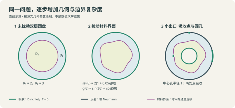



原文:Mean Exit Time。维护与发布:SciML / FiniteVolumeMethod.jl 文档维护者;页面未署个人名。本篇完整翻译原文说明,保留全部推导、参数、32 个代码或输出区块、9 张原站图和文献链接。
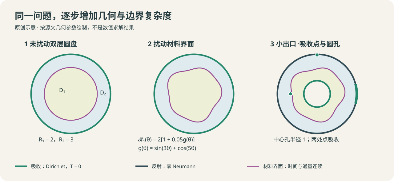
问题定义
本教程讨论平均逃逸时间问题,内容基于原作者此前的一些研究。[1] 对于线性扩散,平均逃逸时间问题通常写成:
D∇2T(x) = −1,x ∈ Ω;
T(x) = 0,x ∈ ∂Ω。 (1)
这里 D 是扩散率。T(x) 表示从位置 x 出发的粒子,经边界 ∂Ω 离开区域所需的平均时间。采用这一解释时,令 D = ℘δ2/(4τ),其中 δ > 0 是粒子的步长,τ > 0 是相邻两步之间的时间间隔,℘ ∈ [0, 1] 是粒子在某个时间步真正发生移动的概率。
在此前的研究中,作者同样采用有限体积法,但把问题写成线性问题,因此求解程序的实现要简单得多。这里介绍的方法则更容易推广到其他非线性问题。
对式(1)的一种更复杂的扩展,是让粒子在非均匀介质中运动,使扩散率随位置 x 变化。具体来说,考虑由两层构成的圆盘 Ω = {0 < r < R1} ∪ {R1 < r < R2},令移动概率 ℘ 在 Ω 内分段为常数,扩散率 D 也相应分段为常数:
P = P1,D = D1,当 0 < r < R1;
P = P2,D = D2,当 R1 < r < R2。
其中 D1 = P1δ2/(4τ),D2 = P2δ2/(4τ)。内区域 0 < r < R1 与外区域 R1 < r < R2 由 r = R1 处的界面分隔。在 r = R2 上施加吸收边界条件,即粒子到达外边界后离开区域。此时,式(1)改写为:
(D1/r) d/dr[r dT(1)/dr] = −1,0 < r < R1;
(D2/r) d/dr[r dT(2)/dr] = −1,R1 < r < R2;
T(1)(R1) = T(2)(R1);
D1(dT(1)/dr)(R1) = D2(dT(2)/dr)(R1);
(dT(1)/dr)(0) = 0;
T(2)(R2) = 0。 (2)
这里采用极坐标,T(1)(r) 是 0 < r < R1 内的平均逃逸时间,T(2)(r) 是 R1 < r < R2 内的平均逃逸时间。界面条件保证 T 及其通量跨界面连续;r = 0 处的 dT(1)/dr = 0 条件则保证 T(1) 在原点有限。这个问题实际上有精确解:
T(1)(r) = (R12 − r2)/(4D1) + (R22 − R12)/(4D2);
T(2)(r) = (R22 − r2)/(4D2)。 (3)
这个精确解稍后会派上用场。
另一种扩展,是让界面不再是简单圆周。引入受扰动的界面 ℛ1(θ),内区域变成 0 < r < ℛ1(θ),外区域变成 ℛ1(θ) < r < R2。将界面函数写成 ℛ1(θ) = R1[1 + εg(θ)],其中 ε ≪ 1 是扰动参数,R1 是未扰动界面的半径,g(θ) 是一个光滑、量级为 O(1)、周期为 2π 的函数。本教程取 g(θ) = sin(3θ) + cos(5θ),ε = 0.05。这样,式(2)变成:
D1∇2T(1)(x) = −1,0 < r < ℛ1(θ);
D2∇2T(2)(x) = −1,ℛ1(θ) < r < R2;
T(1)(ℛ1(θ), θ) = T(2)(ℛ1(θ), θ);
D1∇T(1)(ℛ1(θ), θ) · n̂(θ) = D2∇T(2)(ℛ1(θ), θ) · n̂(θ);
T(2)(R2, θ) = 0。 (4)
原文指出,这个问题没有精确解,但有扰动解;相关推导见 Carr 等(2022)。
教程最后还会进一步修改式(4),在区域中加入空洞,并在原点施加内部 Dirichlet 条件。
未受扰动的界面
先从未受扰动的界面开始求解。虽然式(2)使用 T(1) 和 T(2) 两个变量,因此需要跨界面的连续性方程,但数值上可以用单一变量 T 与随空间变化的扩散率处理。此外,这种数值描述不需要单独添加原点有限性条件。因此,原文将待求问题写为:
D(x)∇2T(x) = −1,x ∈ 𝒟(0, R2);
T(x) = 0,x ∈ ∂𝒟(0, R2)。 (5)
其中,𝒟(0, R2) 是以原点为中心、半径为 R2 的圆盘,且
D(x) = D1,当 ‖x‖ < R1;
D(x) = D2,当 R1 ≤ ‖x‖ ≤ R2。
网格按下面的代码定义。为提高解的精度,在内部圆周附近加入约束边,使该处布置更多三角形。
原文 Julia 代码
using DelaunayTriangulation, FiniteVolumeMethod, CairoMakie
R₁, R₂ = 2.0, 3.0
circle = CircularArc((0.0, R₂), (0.0, R₂), (0.0, 0.0))
points = NTuple{2,Float64}[]
tri = triangulate(points; boundary_nodes=[circle])
θ = LinRange(0, 2π, 250)
xin = @views @. R₁ * cos(θ)[begin:end-1]
yin = @views @. R₁ * sin(θ)[begin:end-1]
add_point!(tri, xin[1], yin[1])
for i in 2:length(xin)
    add_point!(tri, xin[i], yin[i])
    n = DelaunayTriangulation.num_points(tri)
    add_segment!(tri, n - 1, n)
end
n = DelaunayTriangulation.num_points(tri)
add_segment!(tri, n - 1, n)
refine!(tri; max_area=1e-3get_area(tri))
triplot(tri)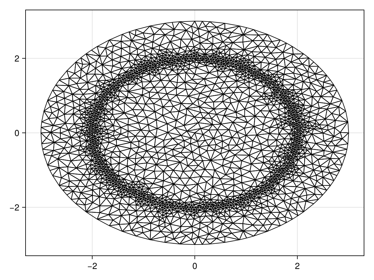
原文 Julia 代码
mesh = FVMGeometry(tri)原文保存的输出(本次未运行)
FVMGeometry with 2035 control volumes, 3978 triangles, and 6012 edges边界条件采用简单的吸收条件。
原文 Julia 代码
BCs = BoundaryConditions(mesh, ((x, y, t, u, p) -> zero(u),), (Dirichlet,))原文保存的输出(本次未运行)
BoundaryConditions with 1 boundary condition with type Dirichlet下面定义问题。首先给出扩散率。
原文 Julia 代码
D₁, D₂ = 6.25e-4, 6.25e-5
diffusion_function = (x, y, t, u, p) -> let r = sqrt(x^2 + y^2)
    return ifelse(r < p.R₁, p.D₁, p.D₂)
end
diffusion_parameters = (R₁=R₁, D₁=D₁, D₂=D₂)
原文保存的输出(本次未运行)
(R₁ = 2.0, D₁ = 0.000625, D₂ = 6.25e-5)接着设置初始条件。请记住,这里所谓的初始条件是稳态求解的初始猜测。我们使用均匀扩散率圆盘的平均逃逸时间精确解,即 (R22 − r2)/(4D2)。
原文 Julia 代码
f = (x, y) -> let r = sqrt(x^2 + y^2)
    return (R₂^2 - r^2) / (4D₂)
end
initial_condition = [f(x, y) for (x, y) in DelaunayTriangulation.each_point(tri)]
原文保存的输出(本次未运行)
2058-element Vector{Float64}:
     0.0
     0.0
     0.0
     0.0
     0.0
     ⋮
 34297.81112014863
  7646.930366955001
 28934.125856402658
 35893.548456787306
 35892.78199272596
现在定义问题。
原文 Julia 代码
source_function = (x, y, t, u, p) -> one(u)
prob = FVMProblem(mesh, BCs;
    diffusion_function, diffusion_parameters,
    source_function, initial_condition,
    final_time=Inf)
原文保存的输出(本次未运行)
FVMProblem with 2035 nodes and time span (0.0, Inf)原文 Julia 代码
steady_prob = SteadyFVMProblem(prob)原文保存的输出(本次未运行)
SteadyFVMProblem with 2035 nodes接下来,像前面的示例一样求解这一问题。
原文 Julia 代码
using SteadyStateDiffEq, LinearSolve, OrdinaryDiffEq
sol = solve(steady_prob, DynamicSS(Rosenbrock23()))
原文保存的输出(本次未运行)
retcode: Success
u: 2058-element Vector{Float64}:
     0.0
     0.0
     0.0
     0.0
     0.0
     ⋮
 21768.966562884172
  7747.4286763664395
 21221.18550088427
 21929.248332073952
 21928.451068967555
原文 Julia 代码
fig = Figure(fontsize=33)
ax = Axis(fig[1, 1], xlabel="x", ylabel="y")
tricontourf!(ax, tri, sol.u, levels=0:500:20000, extendhigh=:auto)
fig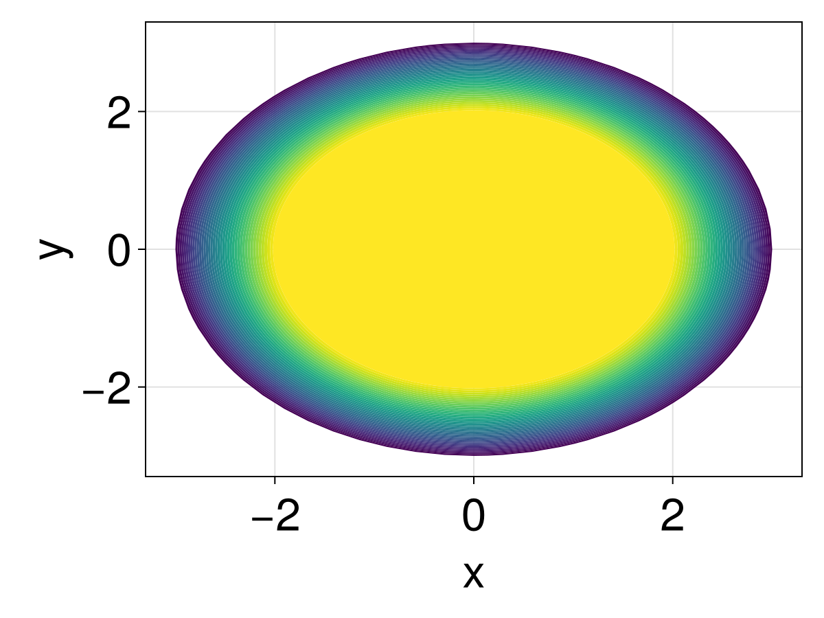
受扰动的界面
现在求解界面受到扰动的情况。网格定义如下。
原文 Julia 代码
g = θ -> sin(3θ) + cos(5θ)
ε = 0.05
R1_f = θ -> R₁ * (1 + ε * g(θ))
points = NTuple{2,Float64}[]
circle = CircularArc((0.0, R₂), (0.0, R₂), (0.0, 0.0))
tri = triangulate(points; boundary_nodes=[circle])
xin = @views (@. R1_f(θ) * cos(θ))[begin:end-1]
yin = @views (@. R1_f(θ) * sin(θ))[begin:end-1]
add_point!(tri, xin[1], yin[1])
for i in 2:length(xin)
    add_point!(tri, xin[i], yin[i])
    n = DelaunayTriangulation.num_points(tri)
    add_segment!(tri, n - 1, n)
end
n = DelaunayTriangulation.num_points(tri)
add_segment!(tri, n - 1, n)
refine!(tri; max_area=1e-3get_area(tri))
triplot(tri)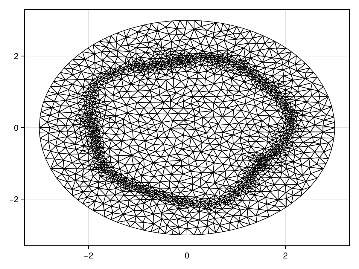
原文 Julia 代码
mesh = FVMGeometry(tri)原文保存的输出(本次未运行)
FVMGeometry with 1863 control volumes, 3621 triangles, and 5483 edges边界条件依然采用简单的吸收条件。
原文 Julia 代码
BCs = BoundaryConditions(mesh, (x, y, t, u, p) -> zero(u), Dirichlet)原文保存的输出(本次未运行)
BoundaryConditions with 1 boundary condition with type Dirichlet下面定义问题。这次使用未扰动界面问题的精确解作为初始条件。
原文 Julia 代码
function T_exact(x, y)
    r = sqrt(x^2 + y^2)
    if r < R₁
        return (R₁^2 - r^2) / (4D₁) + (R₂^2 - R₁^2) / (4D₂)
    else
        return (R₂^2 - r^2) / (4D₂)
    end
end
diffusion_function = (x, y, t, u, p) -> let r = sqrt(x^2 + y^2), θ = atan(y, x)
    interface_val = p.R1_f(θ)
    return ifelse(r < interface_val, p.D₁, p.D₂)
end
diffusion_parameters = (D₁=D₁, D₂=D₂, R1_f=R1_f)
initial_condition = [T_exact(x, y) for (x, y) in DelaunayTriangulation.each_point(tri)]
source_function = (x, y, t, u, p) -> one(u)
prob = FVMProblem(mesh, BCs;
    diffusion_function, diffusion_parameters,
    source_function, initial_condition,
    final_time=Inf)
steady_prob = SteadyFVMProblem(prob)
原文保存的输出(本次未运行)
SteadyFVMProblem with 1863 nodes原文 Julia 代码
sol = solve(steady_prob, DynamicSS(Rosenbrock23()))原文保存的输出(本次未运行)
retcode: Success
u: 1897-element Vector{Float64}:
    0.0
    0.0
    0.0
    0.0
    0.0
    ⋮
 8243.085502168851
 6820.944887685085
 3384.6363956585787
 3707.2375926128075
 3466.633664654742
原文 Julia 代码
fig = Figure(fontsize=33)
ax = Axis(fig[1, 1], xlabel="x", ylabel="y")
tricontourf!(ax, tri, sol.u, levels=0:500:20000, extendhigh=:auto)
lines!(ax, [xin; xin[1]], [yin; yin[1]], color=:magenta, linewidth=5)
fig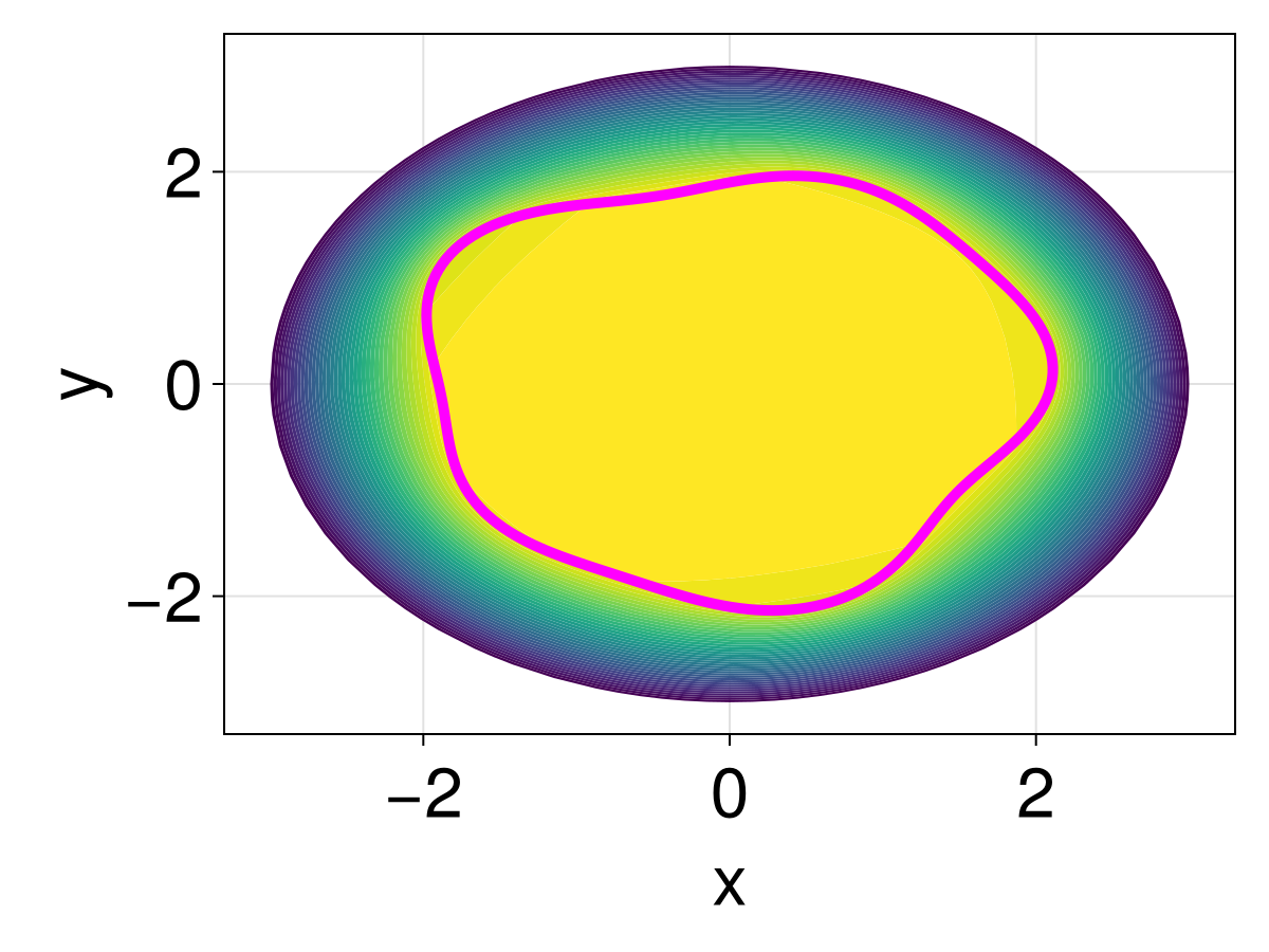
逐步加入吸收点与空洞
现在在问题中加入一些障碍。我们一次增加一个组成部分,分别观察它们的影响。每次修改三角剖分后,都必须更新 mesh,因为它是由先前的 tri 构造的。
首先考虑在原点加入一个点状“孔”。做法是插入原点,再使用 InternalConditions。这个点用来吸收附近的粒子,也就是施加 T(0, 0) = 0。
原文 Julia 代码
add_point!(tri, 0.0, 0.0)
mesh = FVMGeometry(tri)
ICs = InternalConditions((x, y, t, u, p) -> zero(u), dirichlet_nodes=Dict(DelaunayTriangulation.num_points(tri) => 1))
BCs = BoundaryConditions(mesh, (x, y, t, u, p) -> zero(u), Dirichlet)
initial_condition = [T_exact(x, y) for (x, y) in DelaunayTriangulation.each_point(tri)]
prob = FVMProblem(mesh, BCs, ICs;
    diffusion_function, diffusion_parameters,
    source_function, initial_condition,
    final_time=Inf)
steady_prob = SteadyFVMProblem(prob)
sol = solve(steady_prob, DynamicSS(Rosenbrock23()))
fig = Figure(fontsize=33)
ax = Axis(fig[1, 1], xlabel="x", ylabel="y")
tricontourf!(ax, tri, sol.u, levels=0:500:10000, extendhigh=:auto)
lines!(ax, [xin; xin[1]], [yin; yin[1]], color=:magenta, linewidth=5)
fig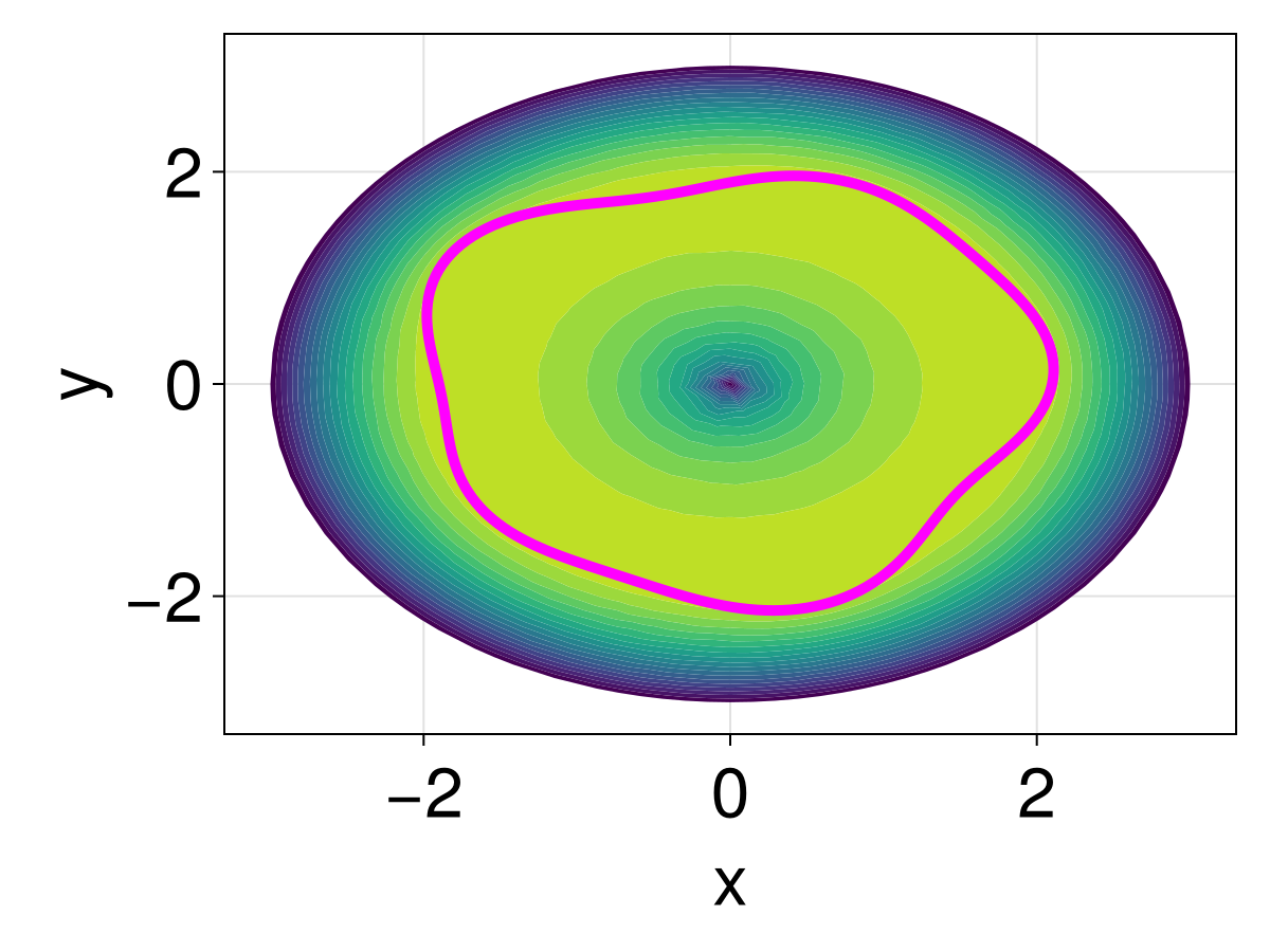
原文图中可以看到,原点的吸收点显著改变了内部时间场。下一步修改外边界:只允许粒子通过其中一小段离开,其余部分都反射粒子。反射边界用 Neumann 边界条件实现。
原文 Julia 代码
ϵr = 0.25
dirichlet_circle = CircularArc((R₂ * cos(ϵr), R₂ * sin(ϵr)), (R₂ * cos(2π - ϵr), R₂ * sin(2π - ϵr)), (0.0, 0.0))
neumann_circle = CircularArc((R₂ * cos(2π - ϵr), R₂ * sin(2π - ϵr)), (R₂ * cos(ϵr), R₂ * sin(ϵr)), (0.0, 0.0))
boundary_nodes = [[dirichlet_circle], [neumann_circle]]
points = NTuple{2,Float64}[]
tri = triangulate(points; boundary_nodes)
xin = @views (@. R1_f(θ) * cos(θ))[begin:end-1]
yin = @views (@. R1_f(θ) * sin(θ))[begin:end-1]
add_point!(tri, xin[1], yin[1])
for i in 2:length(xin)
    add_point!(tri, xin[i], yin[i])
    n = DelaunayTriangulation.num_points(tri)
    add_segment!(tri, n - 1, n)
end
n = DelaunayTriangulation.num_points(tri)
add_segment!(tri, n - 1, n)
add_point!(tri, 0.0, 0.0)
origin_idx = DelaunayTriangulation.num_points(tri)
refine!(tri; max_area=1e-3get_area(tri))
triplot(tri)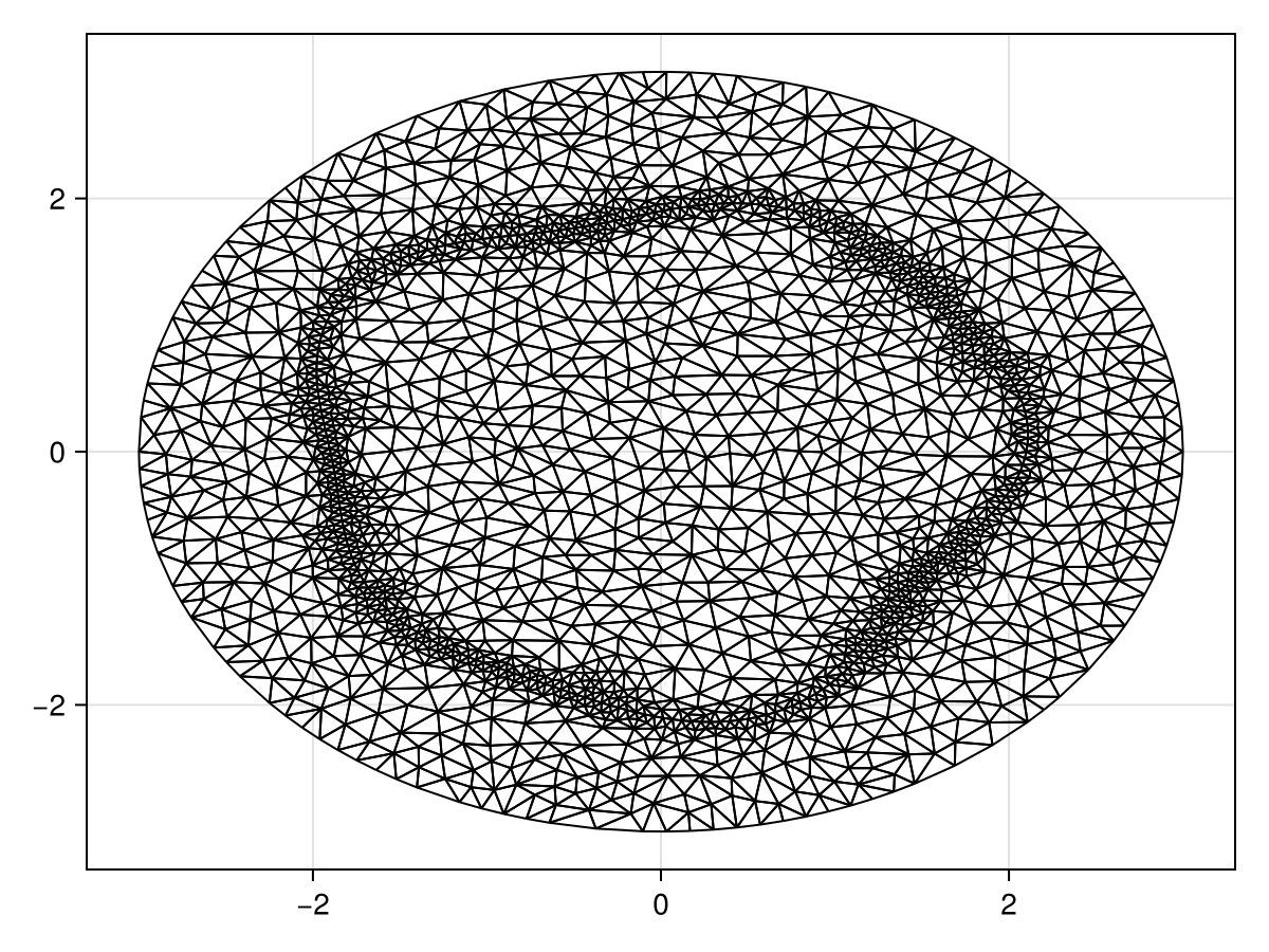
原文 Julia 代码
mesh = FVMGeometry(tri)
zero_f = (x, y, t, u, p) -> zero(u)
BCs = BoundaryConditions(mesh, (zero_f, zero_f), (Neumann, Dirichlet))
ICs = InternalConditions((x, y, t, u, p) -> zero(u), dirichlet_nodes=Dict(origin_idx => 1))
initial_condition = [T_exact(x, y) for (x, y) in DelaunayTriangulation.each_point(tri)]
prob = FVMProblem(mesh, BCs, ICs;
    diffusion_function, diffusion_parameters,
    source_function, initial_condition,
    final_time=Inf)
steady_prob = SteadyFVMProblem(prob)
sol = solve(steady_prob, DynamicSS(Rosenbrock23()))
fig = Figure(fontsize=33)
ax = Axis(fig[1, 1], xlabel="x", ylabel="y")
tricontourf!(ax, tri, sol.u, levels=0:2500:35000, extendhigh=:auto)
lines!(ax, [xin; xin[1]], [yin; yin[1]], color=:magenta, linewidth=5)
fig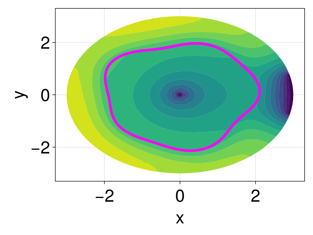
最后再加入一个有面积的空洞:把它放在原点,将原先的点状吸收位置移到 (−2, 0),并在 (0, 2.95) 再加一个点状吸收位置。
原文 Julia 代码
hole = CircularArc((0.0, 1.0), (0.0, 1.0), (0.0, 0.0), positive=false)
boundary_nodes = [[[dirichlet_circle], [neumann_circle]], [[hole]]]
points = NTuple{2,Float64}[]
tri = triangulate(points; boundary_nodes)
xin = @views (@. R1_f(θ) * cos(θ))[begin:end-1]
yin = @views (@. R1_f(θ) * sin(θ))[begin:end-1]
add_point!(tri, xin[1], yin[1])
for i in 2:length(xin)
    add_point!(tri, xin[i], yin[i])
    n = DelaunayTriangulation.num_points(tri)
    add_segment!(tri, n - 1, n)
end
n = DelaunayTriangulation.num_points(tri)
add_segment!(tri, n - 1, n)
add_point!(tri, -2.0, 0.0)
add_point!(tri, 0.0, 2.95)
pointhole_idxs = [DelaunayTriangulation.num_points(tri), DelaunayTriangulation.num_points(tri) - 1]
refine!(tri; max_area=1e-3get_area(tri))
triplot(tri)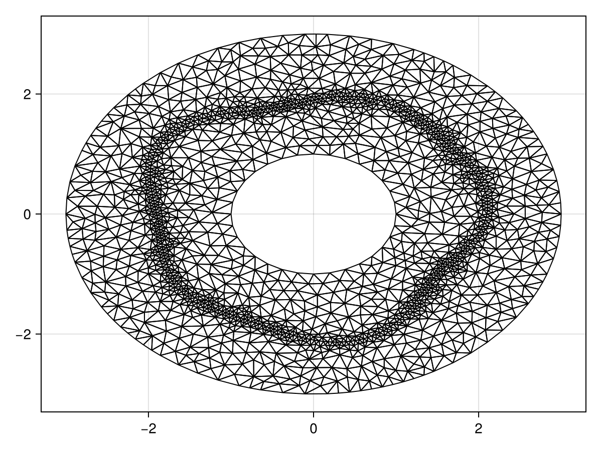
新加入的内部空洞采用吸收边界条件。
原文 Julia 代码
mesh = FVMGeometry(tri)
zero_f = (x, y, t, u, p) -> zero(u)
BCs = BoundaryConditions(mesh, (zero_f, zero_f, zero_f), (Neumann, Dirichlet, Dirichlet))
ICs = InternalConditions((x, y, t, u, p) -> zero(u), dirichlet_nodes=Dict(pointhole_idxs .=> 1))
initial_condition = [T_exact(x, y) for (x, y) in DelaunayTriangulation.each_point(tri)]
prob = FVMProblem(mesh, BCs, ICs;
    diffusion_function, diffusion_parameters,
    source_function, initial_condition,
    final_time=Inf)
steady_prob = SteadyFVMProblem(prob)
sol = solve(steady_prob, DynamicSS(Rosenbrock23()))
fig = Figure(fontsize=33)
ax = Axis(fig[1, 1], xlabel="x", ylabel="y")
tricontourf!(ax, tri, sol.u, levels=0:1000:15000, extendhigh=:auto)
lines!(ax, [xin; xin[1]], [yin; yin[1]], color=:magenta, linewidth=5)
fig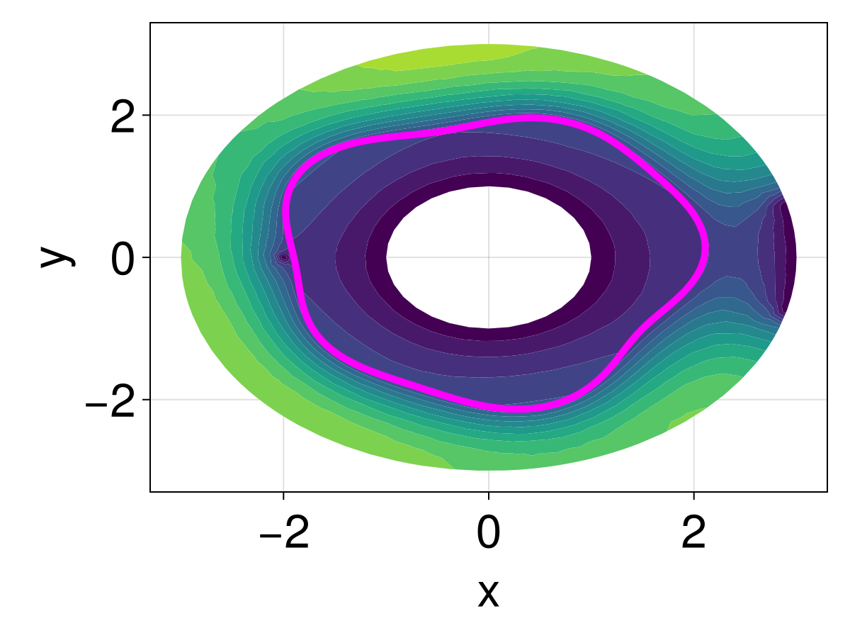
完整代码
以下保留官方完整代码,包括与分步骤展示重复的部分,方便检查变量依赖与执行顺序。它继承前述静态疑点,未经过本地运行修复。
下面给出本例去掉说明文字后的完整代码。也可以查看官方源文件。
原文 Julia 代码
using DelaunayTriangulation, FiniteVolumeMethod, CairoMakie
R₁, R₂ = 2.0, 3.0
circle = CircularArc((0.0, R₂), (0.0, R₂), (0.0, 0.0))
points = NTuple{2,Float64}[]
tri = triangulate(points; boundary_nodes=[circle])
θ = LinRange(0, 2π, 250)
xin = @views @. R₁ * cos(θ)[begin:end-1]
yin = @views @. R₁ * sin(θ)[begin:end-1]
add_point!(tri, xin[1], yin[1])
for i in 2:length(xin)
    add_point!(tri, xin[i], yin[i])
    n = DelaunayTriangulation.num_points(tri)
    add_segment!(tri, n - 1, n)
end
n = DelaunayTriangulation.num_points(tri)
add_segment!(tri, n - 1, n)
refine!(tri; max_area=1e-3get_area(tri))
triplot(tri)

mesh = FVMGeometry(tri)

BCs = BoundaryConditions(mesh, ((x, y, t, u, p) -> zero(u),), (Dirichlet,))

D₁, D₂ = 6.25e-4, 6.25e-5
diffusion_function = (x, y, t, u, p) -> let r = sqrt(x^2 + y^2)
    return ifelse(r < p.R₁, p.D₁, p.D₂)
end
diffusion_parameters = (R₁=R₁, D₁=D₁, D₂=D₂)

f = (x, y) -> let r = sqrt(x^2 + y^2)
    return (R₂^2 - r^2) / (4D₂)
end
initial_condition = [f(x, y) for (x, y) in DelaunayTriangulation.each_point(tri)]

source_function = (x, y, t, u, p) -> one(u)
prob = FVMProblem(mesh, BCs;
    diffusion_function, diffusion_parameters,
    source_function, initial_condition,
    final_time=Inf)

steady_prob = SteadyFVMProblem(prob)

using SteadyStateDiffEq, LinearSolve, OrdinaryDiffEq
sol = solve(steady_prob, DynamicSS(Rosenbrock23()))

fig = Figure(fontsize=33)
ax = Axis(fig[1, 1], xlabel="x", ylabel="y")
tricontourf!(ax, tri, sol.u, levels=0:500:20000, extendhigh=:auto)
fig

g = θ -> sin(3θ) + cos(5θ)
ε = 0.05
R1_f = θ -> R₁ * (1 + ε * g(θ))
points = NTuple{2,Float64}[]
circle = CircularArc((0.0, R₂), (0.0, R₂), (0.0, 0.0))
tri = triangulate(points; boundary_nodes=[circle])
xin = @views (@. R1_f(θ) * cos(θ))[begin:end-1]
yin = @views (@. R1_f(θ) * sin(θ))[begin:end-1]
add_point!(tri, xin[1], yin[1])
for i in 2:length(xin)
    add_point!(tri, xin[i], yin[i])
    n = DelaunayTriangulation.num_points(tri)
    add_segment!(tri, n - 1, n)
end
n = DelaunayTriangulation.num_points(tri)
add_segment!(tri, n - 1, n)
refine!(tri; max_area=1e-3get_area(tri))
triplot(tri)

mesh = FVMGeometry(tri)

BCs = BoundaryConditions(mesh, (x, y, t, u, p) -> zero(u), Dirichlet)

function T_exact(x, y)
    r = sqrt(x^2 + y^2)
    if r < R₁
        return (R₁^2 - r^2) / (4D₁) + (R₂^2 - R₁^2) / (4D₂)
    else
        return (R₂^2 - r^2) / (4D₂)
    end
end
diffusion_function = (x, y, t, u, p) -> let r = sqrt(x^2 + y^2), θ = atan(y, x)
    interface_val = p.R1_f(θ)
    return ifelse(r < interface_val, p.D₁, p.D₂)
end
diffusion_parameters = (D₁=D₁, D₂=D₂, R1_f=R1_f)
initial_condition = [T_exact(x, y) for (x, y) in DelaunayTriangulation.each_point(tri)]
source_function = (x, y, t, u, p) -> one(u)
prob = FVMProblem(mesh, BCs;
    diffusion_function, diffusion_parameters,
    source_function, initial_condition,
    final_time=Inf)
steady_prob = SteadyFVMProblem(prob)

sol = solve(steady_prob, DynamicSS(Rosenbrock23()))

fig = Figure(fontsize=33)
ax = Axis(fig[1, 1], xlabel="x", ylabel="y")
tricontourf!(ax, tri, sol.u, levels=0:500:20000, extendhigh=:auto)
lines!(ax, [xin; xin[1]], [yin; yin[1]], color=:magenta, linewidth=5)
fig

add_point!(tri, 0.0, 0.0)
mesh = FVMGeometry(tri)
ICs = InternalConditions((x, y, t, u, p) -> zero(u), dirichlet_nodes=Dict(DelaunayTriangulation.num_points(tri) => 1))
BCs = BoundaryConditions(mesh, (x, y, t, u, p) -> zero(u), Dirichlet)
initial_condition = [T_exact(x, y) for (x, y) in DelaunayTriangulation.each_point(tri)]
prob = FVMProblem(mesh, BCs, ICs;
    diffusion_function, diffusion_parameters,
    source_function, initial_condition,
    final_time=Inf)
steady_prob = SteadyFVMProblem(prob)
sol = solve(steady_prob, DynamicSS(Rosenbrock23()))
fig = Figure(fontsize=33)
ax = Axis(fig[1, 1], xlabel="x", ylabel="y")
tricontourf!(ax, tri, sol.u, levels=0:500:10000, extendhigh=:auto)
lines!(ax, [xin; xin[1]], [yin; yin[1]], color=:magenta, linewidth=5)
fig

ϵr = 0.25
dirichlet_circle = CircularArc((R₂ * cos(ϵr), R₂ * sin(ϵr)), (R₂ * cos(2π - ϵr), R₂ * sin(2π - ϵr)), (0.0, 0.0))
neumann_circle = CircularArc((R₂ * cos(2π - ϵr), R₂ * sin(2π - ϵr)), (R₂ * cos(ϵr), R₂ * sin(ϵr)), (0.0, 0.0))
boundary_nodes = [[dirichlet_circle], [neumann_circle]]
points = NTuple{2,Float64}[]
tri = triangulate(points; boundary_nodes)
xin = @views (@. R1_f(θ) * cos(θ))[begin:end-1]
yin = @views (@. R1_f(θ) * sin(θ))[begin:end-1]
add_point!(tri, xin[1], yin[1])
for i in 2:length(xin)
    add_point!(tri, xin[i], yin[i])
    n = DelaunayTriangulation.num_points(tri)
    add_segment!(tri, n - 1, n)
end
n = DelaunayTriangulation.num_points(tri)
add_segment!(tri, n - 1, n)
add_point!(tri, 0.0, 0.0)
origin_idx = DelaunayTriangulation.num_points(tri)
refine!(tri; max_area=1e-3get_area(tri))
triplot(tri)

mesh = FVMGeometry(tri)
zero_f = (x, y, t, u, p) -> zero(u)
BCs = BoundaryConditions(mesh, (zero_f, zero_f), (Neumann, Dirichlet))
ICs = InternalConditions((x, y, t, u, p) -> zero(u), dirichlet_nodes=Dict(origin_idx => 1))
initial_condition = [T_exact(x, y) for (x, y) in DelaunayTriangulation.each_point(tri)]
prob = FVMProblem(mesh, BCs, ICs;
    diffusion_function, diffusion_parameters,
    source_function, initial_condition,
    final_time=Inf)
steady_prob = SteadyFVMProblem(prob)
sol = solve(steady_prob, DynamicSS(Rosenbrock23()))
fig = Figure(fontsize=33)
ax = Axis(fig[1, 1], xlabel="x", ylabel="y")
tricontourf!(ax, tri, sol.u, levels=0:2500:35000, extendhigh=:auto)
lines!(ax, [xin; xin[1]], [yin; yin[1]], color=:magenta, linewidth=5)
fig

hole = CircularArc((0.0, 1.0), (0.0, 1.0), (0.0, 0.0), positive=false)
boundary_nodes = [[[dirichlet_circle], [neumann_circle]], [[hole]]]
points = NTuple{2,Float64}[]
tri = triangulate(points; boundary_nodes)
xin = @views (@. R1_f(θ) * cos(θ))[begin:end-1]
yin = @views (@. R1_f(θ) * sin(θ))[begin:end-1]
add_point!(tri, xin[1], yin[1])
for i in 2:length(xin)
    add_point!(tri, xin[i], yin[i])
    n = DelaunayTriangulation.num_points(tri)
    add_segment!(tri, n - 1, n)
end
n = DelaunayTriangulation.num_points(tri)
add_segment!(tri, n - 1, n)
add_point!(tri, -2.0, 0.0)
add_point!(tri, 0.0, 2.95)
pointhole_idxs = [DelaunayTriangulation.num_points(tri), DelaunayTriangulation.num_points(tri) - 1]
refine!(tri; max_area=1e-3get_area(tri))
triplot(tri)

mesh = FVMGeometry(tri)
zero_f = (x, y, t, u, p) -> zero(u)
BCs = BoundaryConditions(mesh, (zero_f, zero_f, zero_f), (Neumann, Dirichlet, Dirichlet))
ICs = InternalConditions((x, y, t, u, p) -> zero(u), dirichlet_nodes=Dict(pointhole_idxs .=> 1))
initial_condition = [T_exact(x, y) for (x, y) in DelaunayTriangulation.each_point(tri)]
prob = FVMProblem(mesh, BCs, ICs;
    diffusion_function, diffusion_parameters,
    source_function, initial_condition,
    final_time=Inf)
steady_prob = SteadyFVMProblem(prob)
sol = solve(steady_prob, DynamicSS(Rosenbrock23()))
fig = Figure(fontsize=33)
ax = Axis(fig[1, 1], xlabel="x", ylabel="y")
tricontourf!(ax, tri, sol.u, levels=0:1000:15000, extendhigh=:auto)
lines!(ax, [xin; xin[1]], [yin; yin[1]], color=:magenta, linewidth=5)
fig
原页面由 Literate.jl 生成。
- 1 参见 Simpson 等(2021)与 Carr 等(2022)。保留原文给出的参考文献链接,未将研究论文作者推定为本教程的个人署名。
复用前的静态核对
修改三角剖分后,重新创建 FVMGeometry,再重建相应边界和内部条件。两个“点状孔”在代码中是设为零值的内部节点,最后的中心圆孔才是从区域中挖去的有面积空洞。三组绘图使用不同等值线级别:不能仅凭颜色深浅跨图定量比较。原文保存的节点数与向量长度也并非一一相等;本次未检查索引机制或网格版本差异,不作未经验证的解释。
本篇可用于理解建模步骤和审查原始实现;是否收敛、界面通量是否正确离散、网格加密后误差如何变化,以及单点吸收条件对结果的影响,都需要在固定依赖环境中另行验证。没有把官方输出当成本地运行证据。
示例代码许可证
随示例代码保留项目版权与许可通知。来源:官方 LICENSE。代码许可与本文其他素材的权利分别适用。
许可全文
MIT License

Copyright (c) 2022 Daniel VandenHeuvel <danj.vandenheuvel@gmail.com>

Permission is hereby granted, free of charge, to any person obtaining a copy of this software and associated documentation files (the "Software"), to deal in the Software without restriction, including without limitation the rights to use, copy, modify, merge, publish, distribute, sublicense, and/or sell copies of the Software, and to permit persons to whom the Software is furnished to do so, subject to the following conditions:

The above copyright notice and this permission notice shall be included in all copies or substantial portions of the Software.

THE SOFTWARE IS PROVIDED "AS IS", WITHOUT WARRANTY OF ANY KIND, EXPRESS OR IMPLIED, INCLUDING BUT NOT LIMITED TO THE WARRANTIES OF MERCHANTABILITY, FITNESS FOR A PARTICULAR PURPOSE AND NONINFRINGEMENT. IN NO EVENT SHALL THE AUTHORS OR COPYRIGHT HOLDERS BE LIABLE FOR ANY CLAIM, DAMAGES OR OTHER LIABILITY, WHETHER IN AN ACTION OF CONTRACT, TORT OR OTHERWISE, ARISING FROM, OUT OF OR IN CONNECTION WITH THE SOFTWARE OR THE USE OR OTHER DEALINGS IN THE SOFTWARE.










暂无评论内容