Matplotlib 标注指南-未完纪

提示

前往页面末尾下载完整示例代码。

标注

标注是图形元素，通常是一段文字，用于解释数据、补充背景，或突出可视化数据中的某一部分。annotate 支持多种坐标系，能灵活设置数据与标注的相对位置，并提供多种文字样式选项。Axes.annotate 还可以添加从文字指向数据的箭头，并以多种方式设置箭头样式。text 也可用于简单的文字标注，但在定位和样式方面不如 annotate 灵活。

基础标注

标注中有两个位置需要考虑：被标注数据的位置 xy，以及标注文字的位置 xytext。这两个参数都是 (x, y) 元组：

import matplotlib.pyplot as plt
import numpy as np

fig, ax = plt.subplots(figsize=(3, 3))

t = np.arange(0.0, 5.0, 0.01)
s = np.cos(2*np.pi*t)
line, = ax.plot(t, s, lw=2)

ax.annotate('local max', xy=(2, 1), xytext=(3, 1.5),
            arrowprops=dict(facecolor='black', shrink=0.05))
ax.set_ylim(-2, 2)

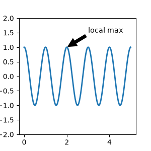
这个示例中的 xy（箭头尖端）和 xytext（文字位置）都采用数据坐标。还可以选择其他多种坐标系：为 xycoords 和 textcoords 指定下表中的字符串，即可设置 xy 和 xytext 的坐标系，默认值为 'data'。

参数	坐标系
'figure points'	相对于 Figure 左下角的点数
'figure pixels'	相对于 Figure 左下角的像素数
'figure fraction'	(0, 0) 为 Figure 左下角，(1, 1) 为右上角
'axes points'	相对于 Axes 左下角的点数
'axes pixels'	相对于 Axes 左下角的像素数
'axes fraction'	(0, 0) 为 Axes 左下角，(1, 1) 为右上角
'data'	使用 Axes 的数据坐标系

下面这些字符串也可作为 textcoords 的参数：

参数	坐标系
'offset points'	相对于 xy 值的偏移量，单位为点
'offset pixels'	相对于 xy 值的偏移量，单位为像素

物理坐标系（点或像素）的原点位于 Figure 或 Axes 的左下角。这里的点是排版点（typographic points），是长度为 1/72 英寸的物理单位。关于点与像素的进一步说明，见物理坐标绘图。

标注数据

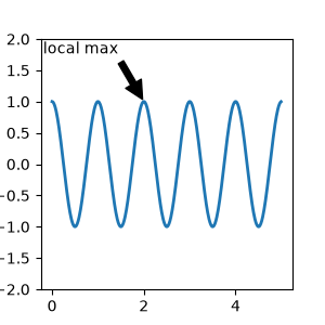
这个示例使用 Axes 的比例坐标指定文字的位置：

fig, ax = plt.subplots(figsize=(3, 3))

t = np.arange(0.0, 5.0, 0.01)
s = np.cos(2*np.pi*t)
line, = ax.plot(t, s, lw=2)

ax.annotate('local max', xy=(2, 1), xycoords='data',
            xytext=(0.01, .99), textcoords='axes fraction',
            va='top', ha='left',
            arrowprops=dict(facecolor='black', shrink=0.05))
ax.set_ylim(-2, 2)

标注 Artist

将某个 Artist 实例作为 xycoords 传入，就可以相对于该 Artist 放置标注。此时 xy 被解释为 Artist 包围框中的比例坐标。

import matplotlib.patches as mpatches

fig, ax = plt.subplots(figsize=(3, 3))
arr = mpatches.FancyArrowPatch((1.25, 1.5), (1.75, 1.5),
                               arrowstyle='->,head_width=.15', mutation_scale=20)
ax.add_patch(arr)
ax.annotate("label", (.5, .5), xycoords=arr, ha='center', va='bottom')
ax.set(xlim=(1, 2), ylim=(1, 2))

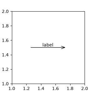
这里的标注位于相对于箭头左下角的 (.5,.5) 位置，水平和垂直位置均以此为参考。垂直方向上，文字底边与参考点对齐，使标签位于线段上方。连续连接多个标注 Artist 的示例，见“标注的坐标系”中的 Artist 小节。

用箭头标注

为可选关键字参数 arrowprops 提供一个箭头属性字典，即可绘制从文字指向被标注点的箭头。

arrowprops 的键	说明
width	箭头宽度，单位为点
frac	箭头头部占箭头总长度的比例
headwidth	箭头头部底边的宽度，单位为点
shrink	使箭头尖端和底部按一定百分比远离被标注点和文字
**kwargs	matplotlib.patches.Polygon 支持的任意键，例如 facecolor

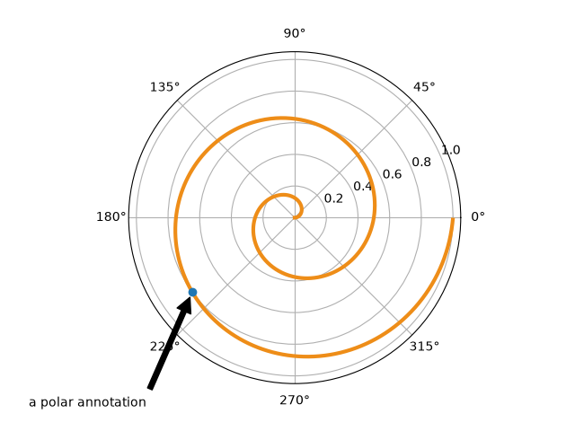
下面示例中的 xy 点使用数据坐标系，因为 xycoords 默认值为 'data'。对于极坐标 Axes，数据坐标为 (theta, radius)。示例中的文字使用 Figure 比例坐标。horizontalalignment、verticalalignment、fontsize 等 matplotlib.text.Text 关键字参数，会由 annotate 传递给 Text 实例。

fig = plt.figure()
ax = fig.add_subplot(projection='polar')
r = np.arange(0, 1, 0.001)
theta = 2 * 2*np.pi * r
line, = ax.plot(theta, r, color='#ee8d18', lw=3)

ind = 800
thisr, thistheta = r[ind], theta[ind]
ax.plot([thistheta], [thisr], 'o')
ax.annotate('a polar annotation',
            xy=(thistheta, thisr),  # theta, radius
            xytext=(0.05, 0.05),    # fraction, fraction
            textcoords='figure fraction',
            arrowprops=dict(facecolor='black', shrink=0.05),
            horizontalalignment='left',
            verticalalignment='bottom')

关于箭头绘图的更多说明，见“自定义标注箭头”。

相对于数据放置文字标注

将 textcoords 关键字参数设为 'offset points' 或 'offset pixels'，即可相对于传入标注的 xy 位置，以偏移量放置标注。

fig, ax = plt.subplots(figsize=(3, 3))
x = [1, 3, 5, 7, 9]
y = [2, 4, 6, 8, 10]
annotations = ["A", "B", "C", "D", "E"]
ax.scatter(x, y, s=20)

for xi, yi, text in zip(x, y, annotations):
    ax.annotate(text,
                xy=(xi, yi), xycoords='data',
                xytext=(1.5, 1.5), textcoords='offset points')

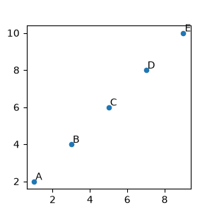
这些标注相对于 xy 值偏移 1.5 点，即 1.5*1/72 英寸。

高级标注

Matplotlib 文档作者建议，在阅读本节之前先阅读“基础标注”、text() 和 annotate()。

带文本框的标注

text 接受 bbox 关键字参数，用于在文字周围绘制文本框：

fig, ax = plt.subplots(figsize=(5, 5))
t = ax.text(0.5, 0.5, "Direction",
            ha="center", va="center", rotation=45, size=15,
            bbox=dict(boxstyle="rarrow,pad=0.3",
                      fc="lightblue", ec="steelblue", lw=2))

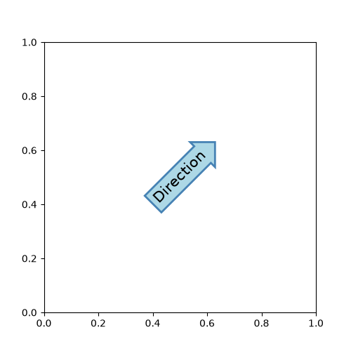
参数包括文本框样式名称，以及作为关键字参数传入的样式属性。目前实现了以下文本框样式：

类	名称	属性
Circle	`circle`	pad=0.3
DArrow	`darrow`	pad=0.3,head_width=1.5,head_angle=90
Ellipse	`ellipse`	pad=0.3
LArrow	`larrow`	pad=0.3,head_width=1.5,head_angle=90
RArrow	`rarrow`	pad=0.3,head_width=1.5,head_angle=90
Round	`round`	pad=0.3,rounding_size=None
Round4	`round4`	pad=0.3,rounding_size=None
Roundtooth	`roundtooth`	pad=0.3,tooth_size=None
Sawtooth	`sawtooth`	pad=0.3,tooth_size=None
Square	`square`	pad=0.3

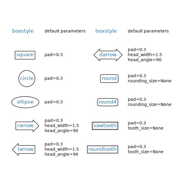
可以通过以下方式访问与文字关联的 patch 对象（文本框）：

bb = t.get_bbox_patch()

返回值是 FancyBboxPatch；可像通常一样访问或修改 facecolor、edgewidth 等 patch 属性。FancyBboxPatch.set_boxstyle 用于设置文本框形状：

bb.set_boxstyle("rarrow", pad=0.6)

也可以在样式名称中用逗号分隔，指定属性参数：

bb.set_boxstyle("rarrow, pad=0.6")

定义自定义文本框样式

自定义文本框样式可实现为一个函数：接收矩形框及“变形”量参数，返回“变形”后的路径。具体函数签名见下方 custom_box_style。

这里返回的新路径在文本框左侧添加了一个“箭头”形状。

之后向 Axes.text 传入 bbox=dict(boxstyle=custom_box_style, …)，即可使用自定义样式。

from matplotlib.path import Path


def custom_box_style(x0, y0, width, height, mutation_size):
    """
    Given the location and size of the box, return the path of the box around it.

    Rotation is automatically taken care of.

    Parameters
    ----------
    x0, y0, width, height : float
       Box location and size.
    mutation_size : float
        Mutation reference scale, typically the text font size.
    """
    # padding
    mypad = 0.3
    pad = mutation_size * mypad
    # width and height with padding added.
    width = width + 2 * pad
    height = height + 2 * pad
    # boundary of the padded box
    x0, y0 = x0 - pad, y0 - pad
    x1, y1 = x0 + width, y0 + height
    # return the new path
    return Path([(x0, y0), (x1, y0), (x1, y1), (x0, y1),
                 (x0-pad, (y0+y1)/2), (x0, y0), (x0, y0)],
                closed=True)

fig, ax = plt.subplots(figsize=(3, 3))
ax.text(0.5, 0.5, "Test", size=30, va="center", ha="center", rotation=30,
        bbox=dict(boxstyle=custom_box_style, alpha=0.2))

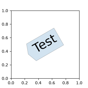
同样，也可以使用实现 __call__ 的类来定义自定义文本框样式。

随后可将这些类注册到 BoxStyle._style_list 字典，从而以字符串形式指定文本框样式：bbox=dict(boxstyle="registered_name,param=value,…", …)。注意，这种注册依赖内部 API，因此并未获得正式支持。

from matplotlib.patches import BoxStyle


class MyStyle:
    """A simple box."""

    def __init__(self, pad=0.3):
        """
        The arguments must be floats and have default values.

        Parameters
        ----------
        pad : float
            amount of padding
        """
        self.pad = pad
        super().__init__()

    def __call__(self, x0, y0, width, height, mutation_size):
        """
        Given the location and size of the box, return the path of the box around it.

        Rotation is automatically taken care of.

        Parameters
        ----------
        x0, y0, width, height : float
            Box location and size.
        mutation_size : float
            Reference scale for the mutation, typically the text font size.
        """
        # padding
        pad = mutation_size * self.pad
        # width and height with padding added
        width = width + 2 * pad
        height = height + 2 * pad
        # boundary of the padded box
        x0, y0 = x0 - pad, y0 - pad
        x1, y1 = x0 + width, y0 + height
        # return the new path
        return Path([(x0, y0), (x1, y0), (x1, y1), (x0, y1),
                     (x0-pad, (y0+y1)/2), (x0, y0), (x0, y0)],
                    closed=True)


BoxStyle._style_list["angled"] = MyStyle  # Register the custom style.

fig, ax = plt.subplots(figsize=(3, 3))
ax.text(0.5, 0.5, "Test", size=30, va="center", ha="center", rotation=30,
        bbox=dict(boxstyle="angled,pad=0.5", alpha=0.2))

del BoxStyle._style_list["angled"]  # Unregister it.

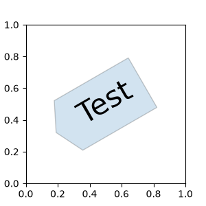
类似地，也可以定义自定义 ConnectionStyle 和 ArrowStyle。查看 patches 源代码，了解各个类的定义方式。

自定义标注箭头

指定 arrowprops 参数，可以选择绘制连接 xy 与 xytext 的箭头。如果只需要绘制箭头，将第一个参数设为空字符串：

fig, ax = plt.subplots(figsize=(3, 3))
ax.annotate("",
            xy=(0.2, 0.2), xycoords='data',
            xytext=(0.8, 0.8), textcoords='data',
            arrowprops=dict(arrowstyle="->", connectionstyle="arc3"))

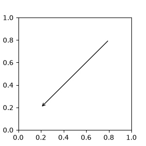
箭头按照以下步骤绘制：

根据 connectionstyle 参数创建连接两个点的路径。
如果设置了 patchA 和 patchB，则裁剪路径，避开这些 patch。
根据 shrinkA 和 shrinkB 进一步缩短路径，单位为像素。
根据 arrowstyle 参数，将路径变换为箭头 patch。

(2x.png, png)

连接两个点的路径由 connectionstyle 键控制，可用样式如下：

名称	属性
`angle`	angleA=90,angleB=0,rad=0.0
`angle3`	angleA=90,angleB=0
`arc`	angleA=0,angleB=0,armA=None,armB=None,rad=0.0
`arc3`	rad=0.0
`bar`	armA=0.0,armB=0.0,fraction=0.3,angle=None

angle3 和 arc3 中的“3”表示生成的路径是一段二次样条，包含三个控制点。如下文所述，一些箭头样式只能用于连接路径为二次样条的情况。

下面的示例有限地展示了各连接样式的行为。警告：bar 样式的行为目前尚未明确定义，未来可能发生变化。

(源代码, 2x.png, png)

标注的连接样式

连接路径经过裁剪和缩短后，再根据指定的 arrowstyle 变形为箭头 patch：

名称	属性
`-`	None
`->`	head_length=0.4,head_width=0.2
`-[`	widthB=1.0,lengthB=0.2,angleB=None
`\|-\|`	widthA=1.0,widthB=1.0
`-\|>`	head_length=0.4,head_width=0.2
`<-`	head_length=0.4,head_width=0.2
`<->`	head_length=0.4,head_width=0.2
`<\|-`	head_length=0.4,head_width=0.2
`<\|-\|>`	head_length=0.4,head_width=0.2
`fancy`	head_length=0.4,head_width=0.4,tail_width=0.4
`simple`	head_length=0.5,head_width=0.5,tail_width=0.2
`wedge`	tail_width=0.3,shrink_factor=0.5

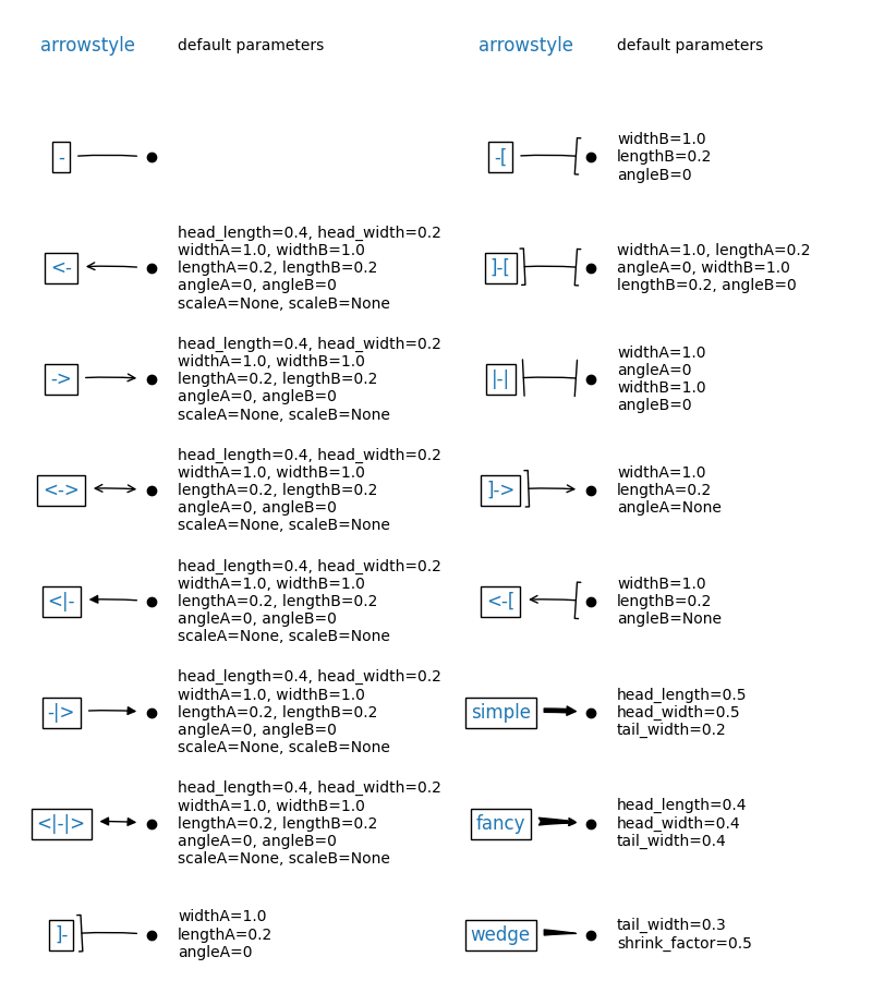
某些 arrowstyles 只适用于生成二次样条段的连接样式，包括 fancy、simple 和 wedge。这些箭头样式必须搭配 "angle3" 或 "arc3" 连接样式。

如果提供了标注字符串，patch 默认设为文字的 bbox patch。

fig, ax = plt.subplots(figsize=(3, 3))

ax.annotate("Test",
            xy=(0.2, 0.2), xycoords='data',
            xytext=(0.8, 0.8), textcoords='data',
            size=20, va="center", ha="center",
            arrowprops=dict(arrowstyle="simple",
                            connectionstyle="arc3,rad=-0.2"))

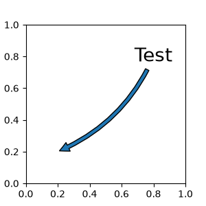
与 text 一样，可以使用 bbox 参数在文字周围绘制文本框。

fig, ax = plt.subplots(figsize=(3, 3))

ann = ax.annotate("Test",
                  xy=(0.2, 0.2), xycoords='data',
                  xytext=(0.8, 0.8), textcoords='data',
                  size=20, va="center", ha="center",
                  bbox=dict(boxstyle="round4", fc="w"),
                  arrowprops=dict(arrowstyle="-|>",
                                  connectionstyle="arc3,rad=-0.2",
                                  fc="w"))

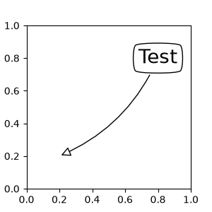
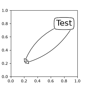
默认的起点设为文字范围的中心。可使用 relpos 键调整该位置，数值按文字范围归一化。例如，(0, 0) 表示左下角，(1, 1) 表示右上角。

fig, ax = plt.subplots(figsize=(3, 3))

ann = ax.annotate("Test",
                  xy=(0.2, 0.2), xycoords='data',
                  xytext=(0.8, 0.8), textcoords='data',
                  size=20, va="center", ha="center",
                  bbox=dict(boxstyle="round4", fc="w"),
                  arrowprops=dict(arrowstyle="-|>",
                                  connectionstyle="arc3,rad=0.2",
                                  relpos=(0., 0.),
                                  fc="w"))

ann = ax.annotate("Test",
                  xy=(0.2, 0.2), xycoords='data',
                  xytext=(0.8, 0.8), textcoords='data',
                  size=20, va="center", ha="center",
                  bbox=dict(boxstyle="round4", fc="w"),
                  arrowprops=dict(arrowstyle="-|>",
                                  connectionstyle="arc3,rad=-0.2",
                                  relpos=(1., 0.),
                                  fc="w"))

在 Axes 的固定位置放置 Artist

有一类 Artist 可以放在 Axes 中的固定位置，常见示例是图例。可使用 OffsetBox 类创建这种 Artist。matplotlib.offsetbox 和 mpl_toolkits.axes_grid1.anchored_artists 中提供了一些预定义类。

from matplotlib.offsetbox import AnchoredText

fig, ax = plt.subplots(figsize=(3, 3))
at = AnchoredText("Figure 1a",
                  prop=dict(size=15), frameon=True, loc='upper left')
at.patch.set_boxstyle("round,pad=0.,rounding_size=0.2")
ax.add_artist(at)

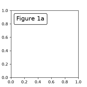
loc 关键字的含义与 legend 命令中的相同。

一个简单应用是：创建 Artist 或一组 Artist 时，已经知道其像素尺寸。例如，要绘制固定为 20 像素 × 20 像素的圆（半径为 10 像素），可以使用 AnchoredDrawingArea。创建实例时指定绘图区的像素尺寸，然后向其中添加任意 Artist。注意，加入绘图区的 Artist 的范围与绘图区本身的放置位置无关，只有初始尺寸起作用。

添加到绘图区的 Artist 不应设置 transform，因为它会被覆盖。这些 Artist 的尺寸按像素坐标解释，即上例中两个圆的半径分别为 10 像素和 5 像素。

from matplotlib.patches import Circle
from mpl_toolkits.axes_grid1.anchored_artists import AnchoredDrawingArea

fig, ax = plt.subplots(figsize=(3, 3))
ada = AnchoredDrawingArea(40, 20, 0, 0,
                          loc='upper right', pad=0., frameon=False)
p1 = Circle((10, 10), 10)
ada.drawing_area.add_artist(p1)
p2 = Circle((30, 10), 5, fc="r")
ada.drawing_area.add_artist(p2)
ax.add_artist(ada)

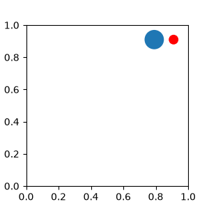
有时希望 Artist 随数据坐标缩放，或随画布像素以外的坐标系缩放。这时可以使用 AnchoredAuxTransformBox 类。它与 AnchoredDrawingArea 类似，但 Artist 的范围会在绘制时，根据指定的 transform 确定。

下面示例中的椭圆，其宽和高分别对应数据坐标中的 0.1 和 0.4；当 Axes 的视图范围变化时，它会自动缩放。

from matplotlib.patches import Ellipse
from mpl_toolkits.axes_grid1.anchored_artists import AnchoredAuxTransformBox

fig, ax = plt.subplots(figsize=(3, 3))
box = AnchoredAuxTransformBox(ax.transData, loc='upper left')
el = Ellipse((0, 0), width=0.1, height=0.4, angle=30)  # in data coordinates!
box.drawing_area.add_artist(el)
ax.add_artist(box)

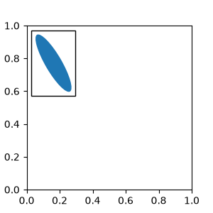
另一种相对于父 Axes 或锚点固定 Artist 的方法，是使用 AnchoredOffsetbox 的 bbox_to_anchor 参数。随后可使用 HPacker 和 VPacker，自动相对于另一 Artist 放置该 Artist：

from matplotlib.offsetbox import (AnchoredOffsetbox, DrawingArea, HPacker,
                                  TextArea)

fig, ax = plt.subplots(figsize=(3, 3))

box1 = TextArea(" Test: ", textprops=dict(color="k"))
box2 = DrawingArea(60, 20, 0, 0)

el1 = Ellipse((10, 10), width=16, height=5, angle=30, fc="r")
el2 = Ellipse((30, 10), width=16, height=5, angle=170, fc="g")
el3 = Ellipse((50, 10), width=16, height=5, angle=230, fc="b")
box2.add_artist(el1)
box2.add_artist(el2)
box2.add_artist(el3)

box = HPacker(children=[box1, box2],
              align="center",
              pad=0, sep=5)

anchored_box = AnchoredOffsetbox(loc='lower left',
                                 child=box, pad=0.,
                                 frameon=True,
                                 bbox_to_anchor=(0., 1.02),
                                 bbox_transform=ax.transAxes,
                                 borderpad=0.,)

ax.add_artist(anchored_box)
fig.subplots_adjust(top=0.8)

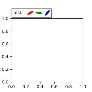
注意，与 Legend 不同，bbox_transform 的默认值为 IdentityTransform。

使用 Artist 作为标注

AnnotationBbox 将 OffsetBox 容器中的 Artist 用作标注，并支持以其他标注方法所用的相同坐标系定位这些标注。更多示例见 Artist 标注示例。

from matplotlib.offsetbox import AnnotationBbox, DrawingArea, OffsetImage
from matplotlib.patches import Annulus

fig, ax = plt.subplots()

text = ax.text(.2, .8, "Green!", color='green')

da = DrawingArea(20, 20)
annulus = Annulus((10, 10), 10, 5, color='tab:green')
da.add_artist(annulus)

# position annulus relative to text
ab1 = AnnotationBbox(da, xy=(.5, 0),
                     xybox=(.5, .25),
                     xycoords=text,
                     boxcoords=(text, "data"),
                     arrowprops=dict(arrowstyle="->"),
                     bboxprops=dict(alpha=0.5))
ax.add_artist(ab1)

N = 25
arr = np.repeat(np.linspace(0, 1, N), N).reshape(N, N)
im = OffsetImage(arr, cmap='Greens')
im.image.axes = ax

# position gradient relative to text and annulus
ab2 = AnnotationBbox(im, xy=(.5, 0),
                     xybox=(.75, 0),
                     xycoords=text,
                     boxcoords=('data', annulus),
                     arrowprops=dict(arrowstyle="->"),
                     bboxprops=dict(alpha=0.5))
ax.add_artist(ab2)

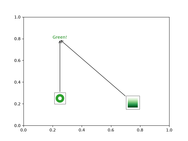
标注的坐标系

Matplotlib 标注支持多种坐标系。“基础标注”中的示例使用数据坐标系。其他一些更高级的选项如下：

Transform 实例

Transform 将坐标映射到不同坐标系，通常映射到显示坐标系。详细解释见坐标变换教程。这里使用 Transform 对象指定对应点的坐标系。例如，Axes.transAxes 变换使标注相对于 Axes 坐标定位，因此等同于将坐标系设为 "axes fraction"：

fig, (ax1, ax2) = plt.subplots(nrows=1, ncols=2, figsize=(6, 3))
ax1.annotate("Test", xy=(0.2, 0.2), xycoords=ax1.transAxes)
ax2.annotate("Test", xy=(0.2, 0.2), xycoords="axes fraction")

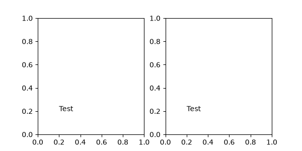
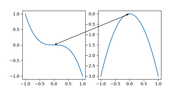
另一个常用的 Transform 实例是 Axes.transData。它对应 Axes 中绘制数据所用的坐标系。这个示例用它在两个 Axes 中相互关联的数据点之间绘制箭头。这里传入空文字，因为标注只是连接数据点。

x = np.linspace(-1, 1)

fig, (ax1, ax2) = plt.subplots(nrows=1, ncols=2, figsize=(6, 3))
ax1.plot(x, -x**3)
ax2.plot(x, -3*x**2)
ax2.annotate("",
             xy=(0, 0), xycoords=ax1.transData,
             xytext=(0, 0), textcoords=ax2.transData,
             arrowprops=dict(arrowstyle="<->"))

Artist 实例

xy 值（或 xytext）被解释为 Artist 包围框 bbox 中的比例坐标：

fig, ax = plt.subplots(nrows=1, ncols=1, figsize=(3, 3))
an1 = ax.annotate("Test 1",
                  xy=(0.5, 0.5), xycoords="data",
                  va="center", ha="center",
                  bbox=dict(boxstyle="round", fc="w"))

an2 = ax.annotate("Test 2",
                  xy=(1, 0.5), xycoords=an1,  # (1, 0.5) of an1's bbox
                  xytext=(30, 0), textcoords="offset points",
                  va="center", ha="left",
                  bbox=dict(boxstyle="round", fc="w"),
                  arrowprops=dict(arrowstyle="->"))

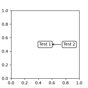
注意，必须确保用作坐标参考的 Artist（本例中为 an1）的范围，在 an2 绘制前已经确定。通常这意味着必须在 an1 之后绘制 an2。所有包围框的基类为 BboxBase。

返回 Transform 或 BboxBase 的可调用对象

这种可调用对象以 renderer 实例为唯一参数，返回 Transform 或 BboxBase。例如，Artist.get_window_extent 返回 bbox，因此使用这个方法等同于第（2）种方式：传入 Artist。

fig, ax = plt.subplots(nrows=1, ncols=1, figsize=(3, 3))
an1 = ax.annotate("Test 1",
                  xy=(0.5, 0.5), xycoords="data",
                  va="center", ha="center",
                  bbox=dict(boxstyle="round", fc="w"))

an2 = ax.annotate("Test 2",
                  xy=(1, 0.5), xycoords=an1.get_window_extent,
                  xytext=(30, 0), textcoords="offset points",
                  va="center", ha="left",
                  bbox=dict(boxstyle="round", fc="w"),
                  arrowprops=dict(arrowstyle="->"))

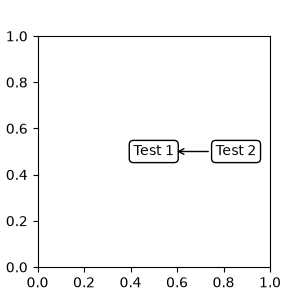
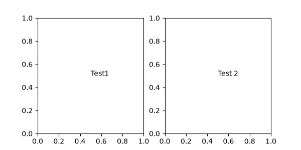
Artist.get_window_extent 给出 Axes 对象的包围框，因此等同于将坐标系设为 axes fraction：

fig, (ax1, ax2) = plt.subplots(nrows=1, ncols=2, figsize=(6, 3))

an1 = ax1.annotate("Test1", xy=(0.5, 0.5), xycoords="axes fraction")
an2 = ax2.annotate("Test 2", xy=(0.5, 0.5), xycoords=ax2.get_window_extent)

混合坐标指定

混合使用一对坐标指定方式：第一个指定 x 坐标，第二个指定 y 坐标。例如，x=0.5 使用数据坐标，y=1 使用归一化 Axes 坐标：

fig, ax = plt.subplots(figsize=(3, 3))
ax.annotate("Test", xy=(0.5, 1), xycoords=("data", "axes fraction"))
ax.axvline(x=.5, color='lightgray')
ax.set(xlim=(0, 2), ylim=(1, 2))

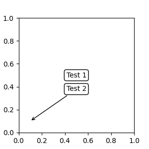
任何受支持的坐标系都可以用于混合指定。例如，文字 "Anchored to 1 & 2" 相对于两个 Text Artist 放置：

fig, ax = plt.subplots(figsize=(3, 3))

t1 = ax.text(0.05, .05, "Text 1", va='bottom', ha='left')
t2 = ax.text(0.90, .90, "Text 2", ha='right')
t3 = ax.annotate("Anchored to 1 & 2", xy=(0, 0), xycoords=(t1, t2),
                 va='bottom', color='tab:orange',)

text.OffsetFrom

有时需要让标注带有一定的 "offset points" 偏移，但偏移的基准并非被标注点，而是其他点或 Artist。text.OffsetFrom 就是为这种情况提供的辅助工具。

from matplotlib.text import OffsetFrom

fig, ax = plt.subplots(figsize=(3, 3))
an1 = ax.annotate("Test 1", xy=(0.5, 0.5), xycoords="data",
                  va="center", ha="center",
                  bbox=dict(boxstyle="round", fc="w"))

offset_from = OffsetFrom(an1, (0.5, 0))
an2 = ax.annotate("Test 2", xy=(0.1, 0.1), xycoords="data",
                  xytext=(0, -10), textcoords=offset_from,
                  # xytext is offset points from "xy=(0.5, 0), xycoords=an1"
                  va="top", ha="center",
                  bbox=dict(boxstyle="round", fc="w"),
                  arrowprops=dict(arrowstyle="->"))

非文字标注

使用 ConnectionPatch

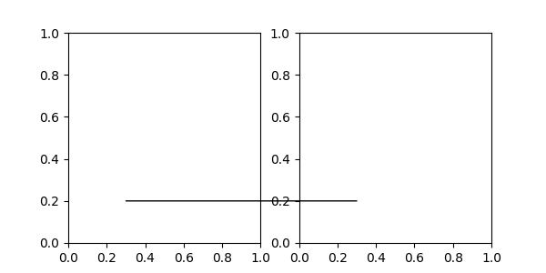
ConnectionPatch 类似于不带文字的标注。annotate 足以应对大多数情况；当需要连接不同 Axes 中的点时，ConnectionPatch 很有用。例如，这里将 ax1 数据坐标中的 xy 点，连接到 ax2 数据坐标中的 xy 点：

from matplotlib.patches import ConnectionPatch

fig, (ax1, ax2) = plt.subplots(nrows=1, ncols=2, figsize=(6, 3))
xy = (0.3, 0.2)
con = ConnectionPatch(xyA=xy, coordsA=ax1.transData,
                      xyB=xy, coordsB=ax2.transData)

fig.add_artist(con)

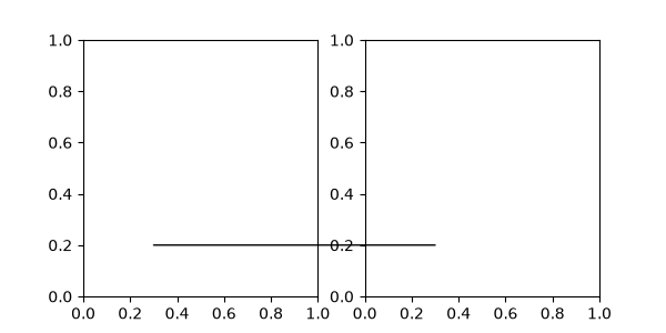
这里通过 add_artist 将 ConnectionPatch 添加到 Figure，而不是某个 Axes。这确保 ConnectionPatch Artist 绘制在两个 Axes 的上方；使用 constrained_layout 布置 Axes 时，也必须采用这种方式。

Axes 之间的缩放效果

mpl_toolkits.axes_grid1.inset_locator 定义了一些可用于连接两个 Axes 的 patch 类。

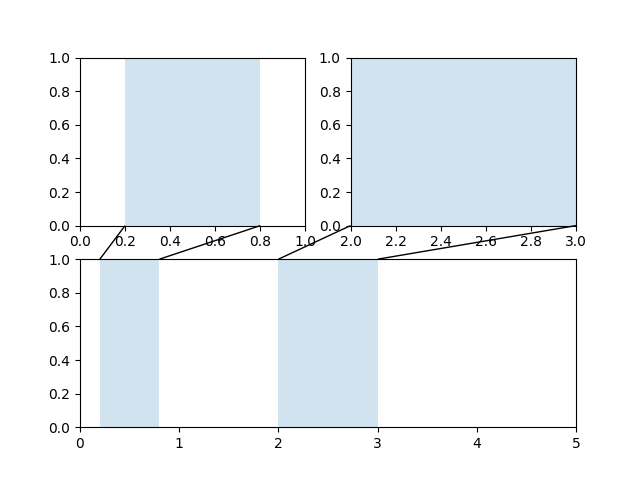
这张图的代码见 Axes 缩放效果。Matplotlib 文档作者建议先熟悉坐标变换教程。

官方脚本总运行时间：（0 分 6.873 秒）

下载 Jupyter notebook：annotations.ipynb

下载 Python 源代码：annotations.py

下载压缩包：annotations.zip

示例图库由 Sphinx-Gallery 生成

来源与许可

License agreement for matplotlib versions 1.3.0 and later
=========================================================

1. This LICENSE AGREEMENT is between the Matplotlib Development Team
("MDT"), and the Individual or Organization ("Licensee") accessing and
otherwise using matplotlib software in source or binary form and its
associated documentation.

2. Subject to the terms and conditions of this License Agreement, MDT
hereby grants Licensee a nonexclusive, royalty-free, world-wide license
to reproduce, analyze, test, perform and/or display publicly, prepare
derivative works, distribute, and otherwise use matplotlib
alone or in any derivative version, provided, however, that MDT's
License Agreement and MDT's notice of copyright, i.e., "Copyright (c)
2012- Matplotlib Development Team; All Rights Reserved" are retained in
matplotlib  alone or in any derivative version prepared by
Licensee.

3. In the event Licensee prepares a derivative work that is based on or
incorporates matplotlib or any part thereof, and wants to
make the derivative work available to others as provided herein, then
Licensee hereby agrees to include in any such work a brief summary of
the changes made to matplotlib .

4. MDT is making matplotlib available to Licensee on an "AS
IS" basis.  MDT MAKES NO REPRESENTATIONS OR WARRANTIES, EXPRESS OR
IMPLIED.  BY WAY OF EXAMPLE, BUT NOT LIMITATION, MDT MAKES NO AND
DISCLAIMS ANY REPRESENTATION OR WARRANTY OF MERCHANTABILITY OR FITNESS
FOR ANY PARTICULAR PURPOSE OR THAT THE USE OF MATPLOTLIB
WILL NOT INFRINGE ANY THIRD PARTY RIGHTS.

5. MDT SHALL NOT BE LIABLE TO LICENSEE OR ANY OTHER USERS OF MATPLOTLIB
 FOR ANY INCIDENTAL, SPECIAL, OR CONSEQUENTIAL DAMAGES OR
LOSS AS A RESULT OF MODIFYING, DISTRIBUTING, OR OTHERWISE USING
MATPLOTLIB , OR ANY DERIVATIVE THEREOF, EVEN IF ADVISED OF
THE POSSIBILITY THEREOF.

6. This License Agreement will automatically terminate upon a material
breach of its terms and conditions.

7. Nothing in this License Agreement shall be deemed to create any
relationship of agency, partnership, or joint venture between MDT and
Licensee.  This License Agreement does not grant permission to use MDT
trademarks or trade name in a trademark sense to endorse or promote
products or services of Licensee, or any third party.

8. By copying, installing or otherwise using matplotlib ,
Licensee agrees to be bound by the terms and conditions of this License
Agreement.

License agreement for matplotlib versions prior to 1.3.0
========================================================

1. This LICENSE AGREEMENT is between John D. Hunter ("JDH"), and the
Individual or Organization ("Licensee") accessing and otherwise using
matplotlib software in source or binary form and its associated
documentation.

2. Subject to the terms and conditions of this License Agreement, JDH
hereby grants Licensee a nonexclusive, royalty-free, world-wide license
to reproduce, analyze, test, perform and/or display publicly, prepare
derivative works, distribute, and otherwise use matplotlib
alone or in any derivative version, provided, however, that JDH's
License Agreement and JDH's notice of copyright, i.e., "Copyright (c)
2002-2011 John D. Hunter; All Rights Reserved" are retained in
matplotlib  alone or in any derivative version prepared by
Licensee.

3. In the event Licensee prepares a derivative work that is based on or
incorporates matplotlib  or any part thereof, and wants to
make the derivative work available to others as provided herein, then
Licensee hereby agrees to include in any such work a brief summary of
the changes made to matplotlib.

4. JDH is making matplotlib  available to Licensee on an "AS
IS" basis.  JDH MAKES NO REPRESENTATIONS OR WARRANTIES, EXPRESS OR
IMPLIED.  BY WAY OF EXAMPLE, BUT NOT LIMITATION, JDH MAKES NO AND
DISCLAIMS ANY REPRESENTATION OR WARRANTY OF MERCHANTABILITY OR FITNESS
FOR ANY PARTICULAR PURPOSE OR THAT THE USE OF MATPLOTLIB
WILL NOT INFRINGE ANY THIRD PARTY RIGHTS.

5. JDH SHALL NOT BE LIABLE TO LICENSEE OR ANY OTHER USERS OF MATPLOTLIB
 FOR ANY INCIDENTAL, SPECIAL, OR CONSEQUENTIAL DAMAGES OR
LOSS AS A RESULT OF MODIFYING, DISTRIBUTING, OR OTHERWISE USING
MATPLOTLIB , OR ANY DERIVATIVE THEREOF, EVEN IF ADVISED OF
THE POSSIBILITY THEREOF.

6. This License Agreement will automatically terminate upon a material
breach of its terms and conditions.

7. Nothing in this License Agreement shall be deemed to create any
relationship of agency, partnership, or joint venture between JDH and
Licensee.  This License Agreement does not grant permission to use JDH
trademarks or trade name in a trademark sense to endorse or promote
products or services of Licensee, or any third party.

8. By copying, installing or otherwise using matplotlib,
Licensee agrees to be bound by the terms and conditions of this License
Agreement.

文章版权归作者所有，未经允许请勿转载。

THE END